<?xml version="1.0" encoding="utf-8"?><feed xmlns="http://www.w3.org/2005/Atom" ><generator uri="https://jekyllrb.com/" version="3.10.0">Jekyll</generator><link href="https://chae-sy.github.io/feed.xml" rel="self" type="application/atom+xml" /><link href="https://chae-sy.github.io/" rel="alternate" type="text/html" /><updated>2026-08-07T02:24:52+00:00</updated><id>https://chae-sy.github.io/feed.xml</id><title type="html">Seoyoon Chae</title><subtitle>Master&apos;s student working on efficient deep learning systems, model compression, and hardware-aware AI accelerators.</subtitle><author><name>Seoyoon Chae</name><email>sychaeee@g.skku.edu</email></author><entry><title type="html">[SSE3021 Digital Integrated Circuit Design] Schematic and Layout Design of 16x16bit 6T SRAM</title><link href="https://chae-sy.github.io/SRAM/" rel="alternate" type="text/html" title="[SSE3021 Digital Integrated Circuit Design] Schematic and Layout Design of 16x16bit 6T SRAM" /><published>2026-06-21T00:00:00+00:00</published><updated>2026-06-21T00:00:00+00:00</updated><id>https://chae-sy.github.io/SRAM</id><content type="html" xml:base="https://chae-sy.github.io/SRAM/"><![CDATA[<p>This is the report submitted to Digital Integrated Circuit Design course (2026 Spring semester SSE3021, SKKU).</p>

<h1 id="1-6t-sram-cell-design">1. 6T SRAM Cell Design</h1>

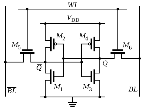
<p><img src="/images/2026-06-21/SRAM_Cell.png" alt="Fig.1 : SRAM Cell" /></p>

<p>Fig.1 : SRAM Cell</p>

<p>This shows a standard 6T SRAM cell composed of six transistors: two cross-coupled CMOS inverters for data storage and two access transistors controlled by the wordline (WL). The cell stores one bit of data by maintaining complementary internal nodes (Q and QB), while the bitlines (BL and BLB) are used for read and write operations. This structure provides fast access, low static power consumption, and robust data retention, making it the most widely used SRAM cell architecture.</p>

<h2 id="schematic">Schematic</h2>

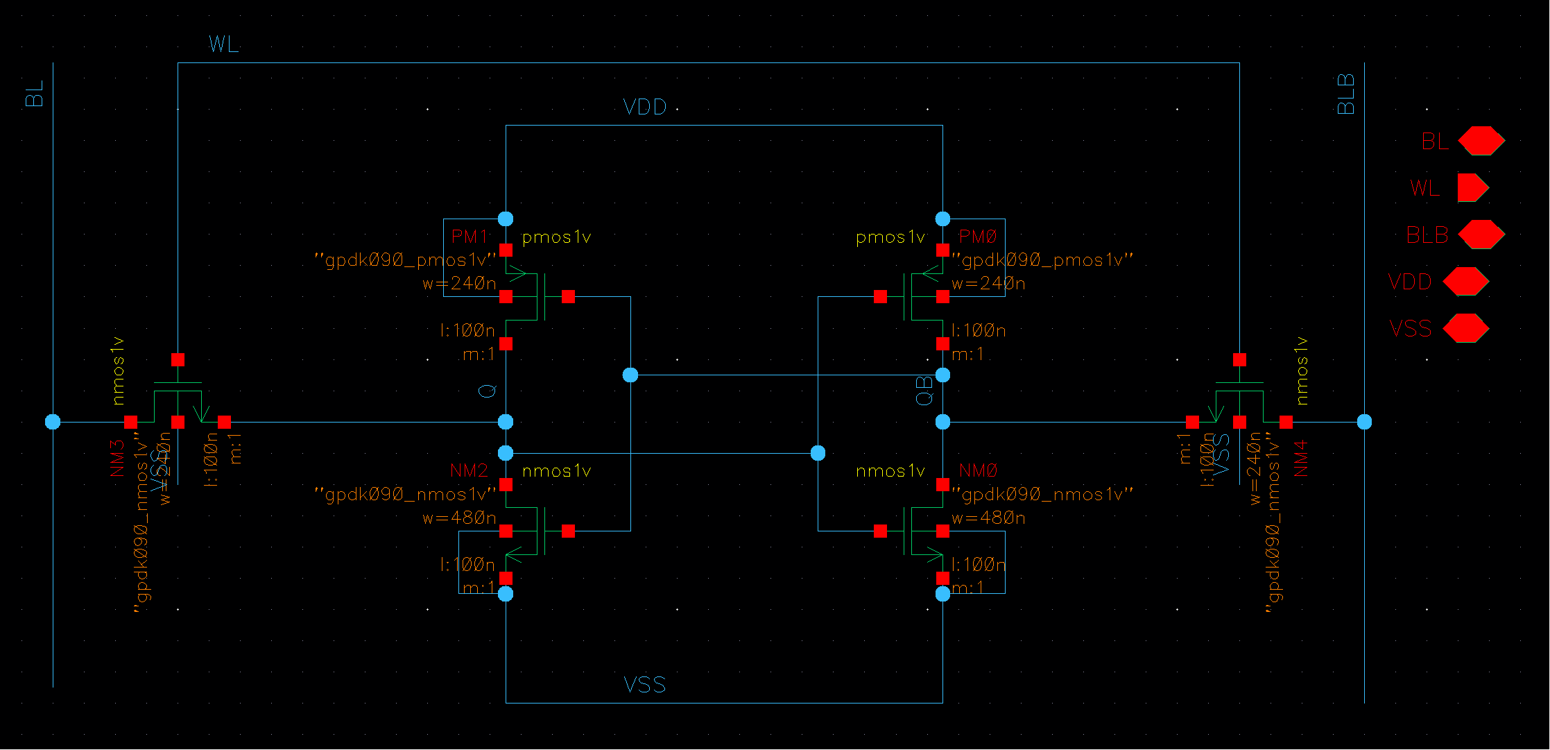
<p><img src="/images/2026-06-21/SRAM_cell_s.png" alt="Fig.2 : SRAM Cell Schematic" /></p>

<p>Fig.2 : SRAM Cell Schematic</p>

<p>Based on the standard 6T SRAM architecture, the schematic was implemented using two cross-coupled CMOS inverters and two access transistors. The cell stores data at nodes Q and QB, while BL, BLB, and WL are used for read and write operations.</p>

<h2 id="functionality-verification">Functionality Verification</h2>

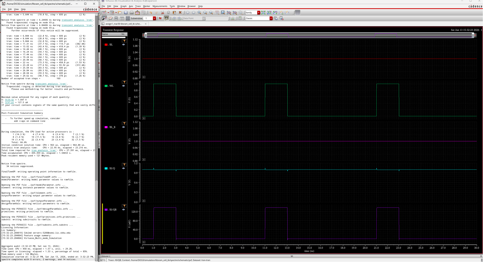
<p><img src="/images/2026-06-21/read.png" alt="Fig.3 : Read" /></p>

<p>Fig.3 : Read Verification</p>

<p>The read operation was successfully verified, as the stored data remained unchanged during the read access while WL was asserted and both bitlines were precharged to VDD.</p>

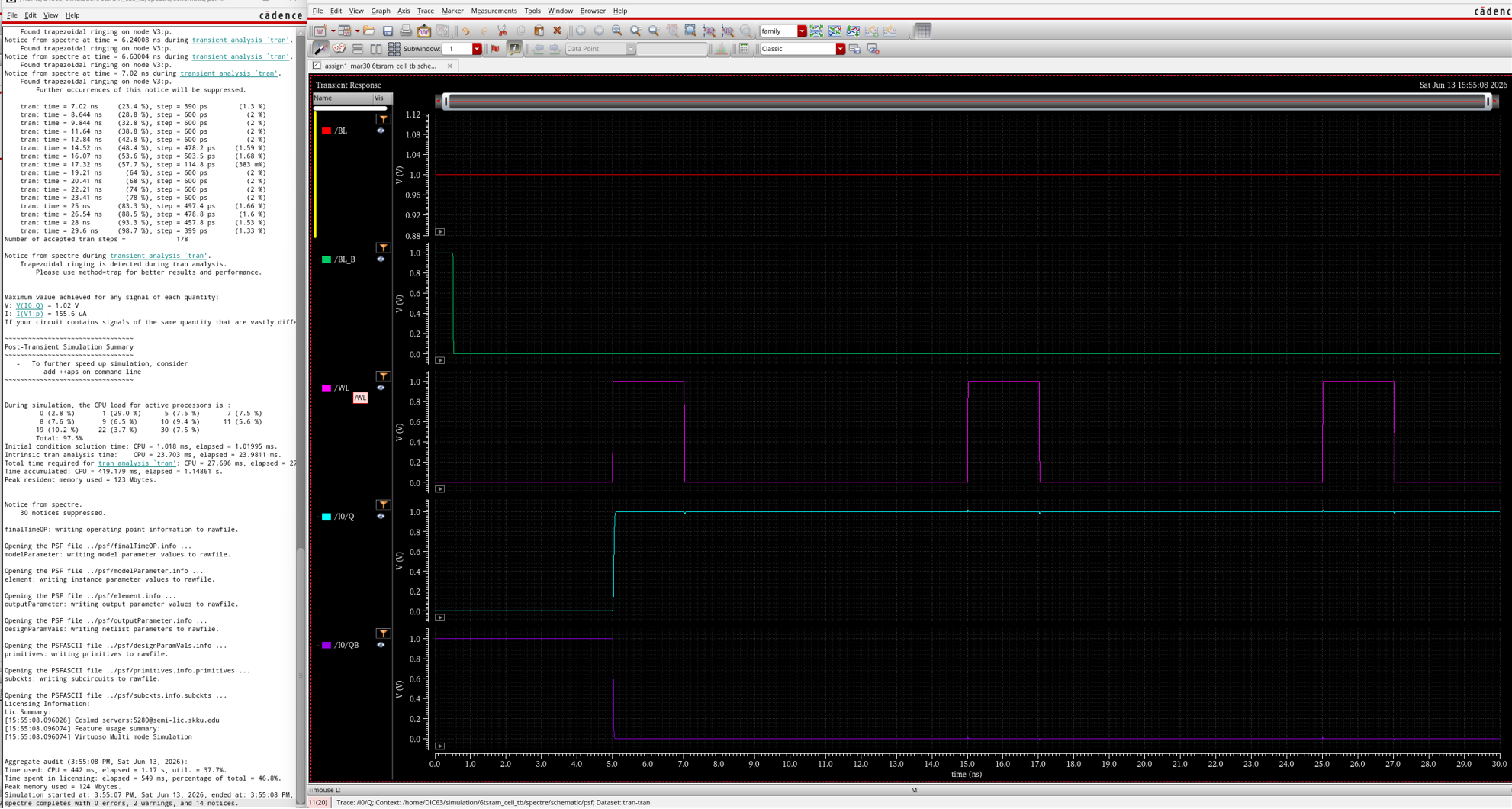
<p><img src="/images/2026-06-21/write.png" alt="Fig.4 : Write" /></p>

<p>Fig.4 : Write Verification</p>

<p>The write operation was successfully verified, as the stored data changed from (Q, QB) = (1, 0) to (0, 1) when WL was asserted with BL = 0 and BLB = 1.</p>

<h2 id="static-noise-margin">Static Noise Margin</h2>

<p><img src="/images/2026-06-21/snm.png" alt="Fig.5 : SNM" /></p>

<p>Fig.5 : Static Noise Margin</p>

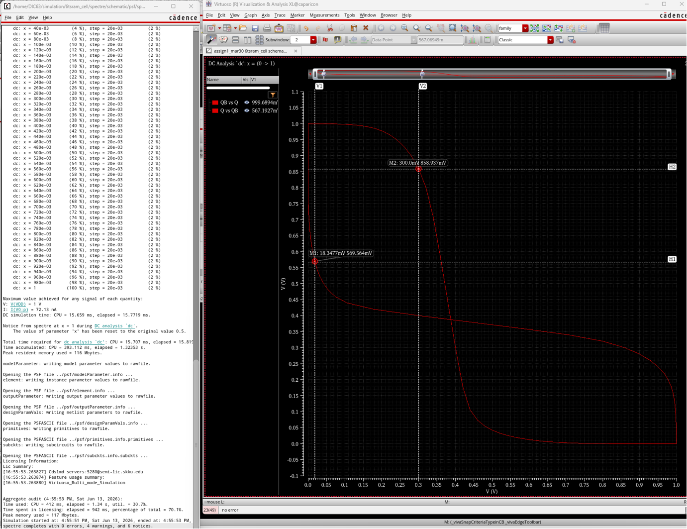
<p>The hold static noise margin (SNM) of the designed 6T SRAM cell was measured to be approximately 282 mV from the butterfly curve, indicating stable data retention in the hold state.</p>

<h1 id="2-sram-column-design">2. SRAM Column Design</h1>

<h2 id="4-to-16-decoder-with-enable-signal">4-to-16 Decoder with Enable Signal</h2>

<p>The 4-to-16 decoder is used as the row decoder in the 16×16 SRAM array. Since the array contains 16 rows, four address bits are required to uniquely select one row. The decoder converts the 4-bit row address into one of sixteen wordline signals (WL0–WL15), ensuring that only the selected row is activated during read or write operations. Without the decoder, it would not be possible to access an individual row within the SRAM array. Therefore, the 4-to-16 decoder is an essential component that enables correct row selection and memory access in the 16×16 SRAM design.</p>

<p><img src="/images/2026-06-21/2-to-4-decoder.png" alt="Fig.6 : 2-to-4 decoder" /></p>

<p>Fig.6 : 2:4 Decoder</p>

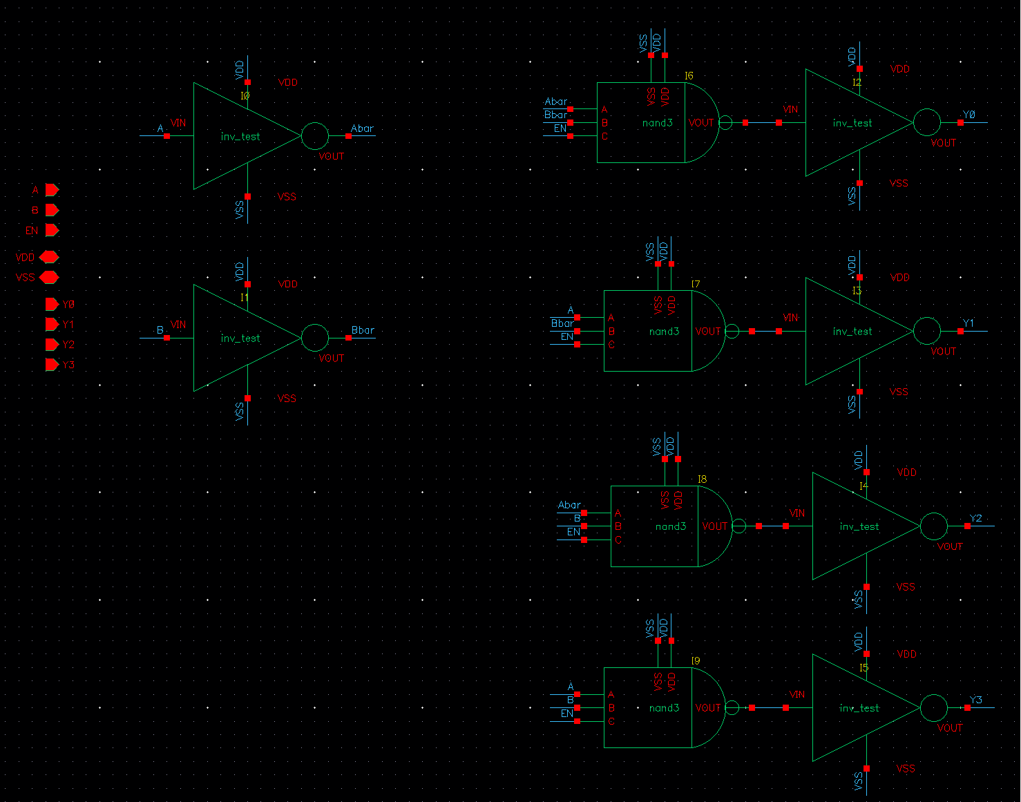
<p>As a building block for the 4-to-16 decoder, a 2-to-4 decoder was first designed and implemented. The schematic is shown above.</p>

<p><img src="/images/2026-06-21/4-to-16-decoder.png" alt="Fig.7 : 4-to-16 decoder" /></p>

<p>Fig.7 : 4:16 Decoder</p>

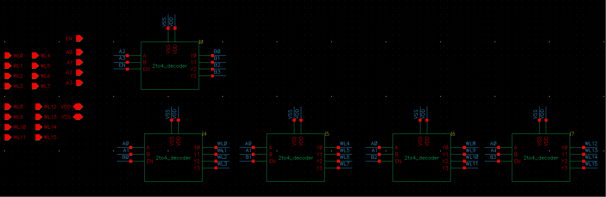
<p>To implement the 4-to-16 decoder, a hierarchical structure based on five 2-to-4 decoders was used. As shown in the schematic, the upper 2-to-4 decoder receives the two most significant address bits (A3 and A2) and generates four enable signals (B0–B3). These enable signals are connected to the enable inputs of four lower 2-to-4 decoders. Each lower decoder receives the two least significant address bits (A1 and A0) and generates four wordline outputs. As a result, only one of the sixteen outputs (WL0–WL15) is asserted for a given 4-bit address, realizing a complete 4-to-16 decoding function.</p>

<h2 id="bit-line-sense-amplifier-blsa">Bit Line Sense Amplifier (BLSA)</h2>

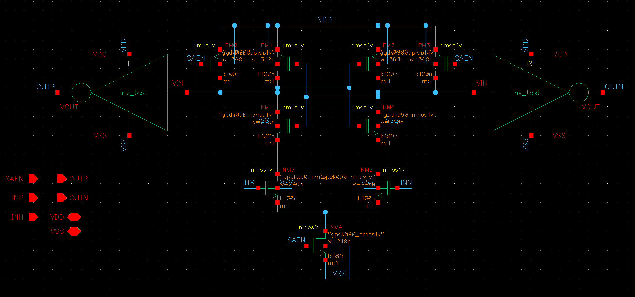
<p><img src="/images/2026-06-21/blsa.png" alt="Fig.8 : BLSA" /></p>

<p>Fig.8 : BLSA</p>

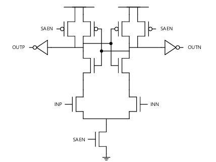
<p>The Bit-Line Sense Amplifier (BLSA) detects a small voltage difference between INP and INN and amplifies it to full-swing digital outputs. When SAEN is low, the sensing circuit is disabled. When SAEN is asserted, the differential input pair converts the input voltage difference into a current difference. The cross-coupled latch then provides positive feedback, rapidly amplifying the small input difference until one output is driven to logic high and the other to logic low. As a result, even a 100 mV input difference can be reliably sensed and converted into complementary outputs (OUTP and OUTN).
In an SRAM array, the BLSA is essential because the read operation produces only a small voltage difference on the bitlines, which must be amplified into full-swing digital signals for reliable data sensing.</p>

<p><img src="/images/2026-06-21/blsa_s.png" alt="Fig.9 : BLSA Schematic" /></p>

<p>Fig.9 : BLSA Schematic</p>

<p>The BLSA schematic was designed as shown above for reliable sensing of bitline voltage differences in the SRAM array.</p>

<h2 id="write-driver-and-precharge">Write Driver and Precharge</h2>

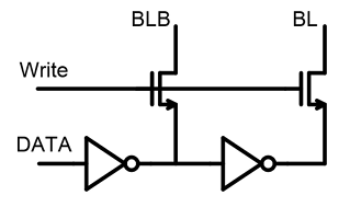
<p><img src="/images/2026-06-21/write_driver.png" alt="Fig.10 : Write Driver" /></p>

<p>Fig.10 : Write Driver</p>

<p>The write driver is a circuit that drives the bitlines (BL and BLB) with complementary data values during a write operation. As shown above, when the Write signal is asserted, the write driver forces BL and BLB to opposite logic levels according to the input DATA, allowing the selected SRAM cell to be overwritten with the new value.</p>

<p>In an SRAM array, the write driver is essential because the cross-coupled inverters inside the SRAM cell are designed to strongly hold their stored data. Therefore, the bitlines must be actively driven to the desired logic levels with sufficient strength to overcome the stored value and successfully write new data into the selected cell. Without a write driver, reliable write operations would not be possible.</p>

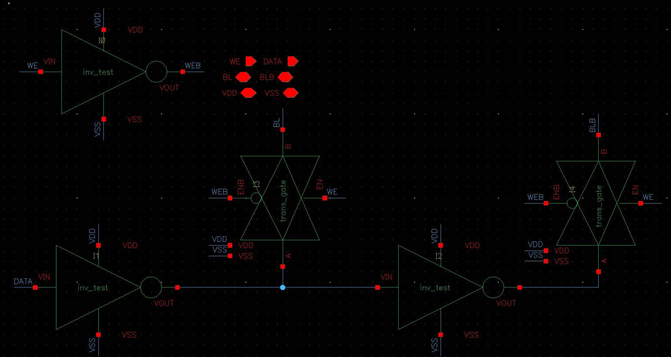
<p><img src="/images/2026-06-21/write_driver_s.png" alt="Fig.11 : Write Driver Schematic" /></p>

<p>Fig.11 : Write Driver Schematic</p>

<p>Instead of using a single NMOS pass transistor, transmission gates were employed in the write driver to achieve full voltage swing on the bitlines. A single NMOS suffers from a threshold-voltage drop when passing a logic high level, resulting in a degraded output voltage. In contrast, a transmission gate combines an NMOS and a PMOS, enabling both strong logic ‘1’ and strong logic ‘0’ transmission. Therefore, the proposed design can drive BL and BLB closer to the full VDD and GND levels, improving write reliability.</p>

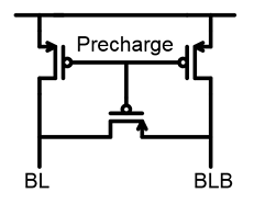
<p><img src="/images/2026-06-21/precharge.png" alt="Fig.12 : Precharge Circuit" /></p>

<p>Fig.12 : Precharge Circuit</p>

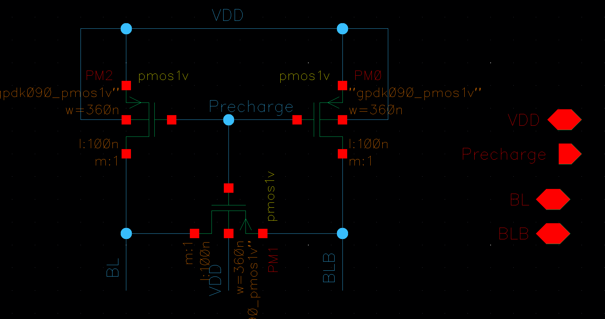
<p>The precharge circuit initializes both bitlines (BL and BLB) to VDD and equalizes their voltages before a read operation. When the Precharge signal is asserted, both bitlines are charged to the same voltage level.
In an SRAM array, the precharge circuit is essential because it provides a known initial condition for the bitlines, allowing the sense amplifier to accurately detect the small voltage difference generated during a read operation.</p>

<p><img src="/images/2026-06-21/precharge_s.png" alt="Fig.13 : Precharge Schematic" /></p>

<p>Fig.13 : Precharge Schematic</p>

<p>The precharge circuit shown above was designed to precharge and equalize BL and BLB before each read operation, enabling reliable sensing in the SRAM array.</p>

<h2 id="1-column-with-16bit-sram-cell">1 Column with 16bit SRAM cell</h2>

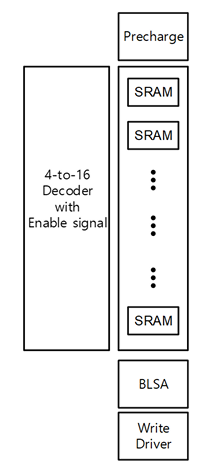
<p><img src="/images/2026-06-21/sram_1col.png" alt="Fig.14 : SRAM Column" /></p>

<p>Fig.14 : SRAM Column</p>

<p>As shown in the figure, a single SRAM column consists of several key components:</p>

<p><strong>4-to-16 Decoder</strong>: Selects one of the sixteen wordlines (WLs) based on the input address.
SRAM Cells: Sixteen 6T SRAM cells are connected vertically in the column. Each cell shares the same bitline pair (BL and BLB) but has a different wordline.</p>

<p><strong>Precharge Circuit</strong>: Precharges and equalizes BL and BLB before every read operation.</p>

<p><strong>Write Driver</strong>: Drives BL and BLB with complementary data values during write operations.
Bit-Line Sense Amplifier (BLSA): Detects and amplifies the small voltage difference developed on BL and BLB during read operations.</p>

<p>During operation, the decoder activates a single wordline, allowing one SRAM cell to communicate with the shared bitlines. The write driver is used for write operations, while the BLSA is used for read operations.</p>

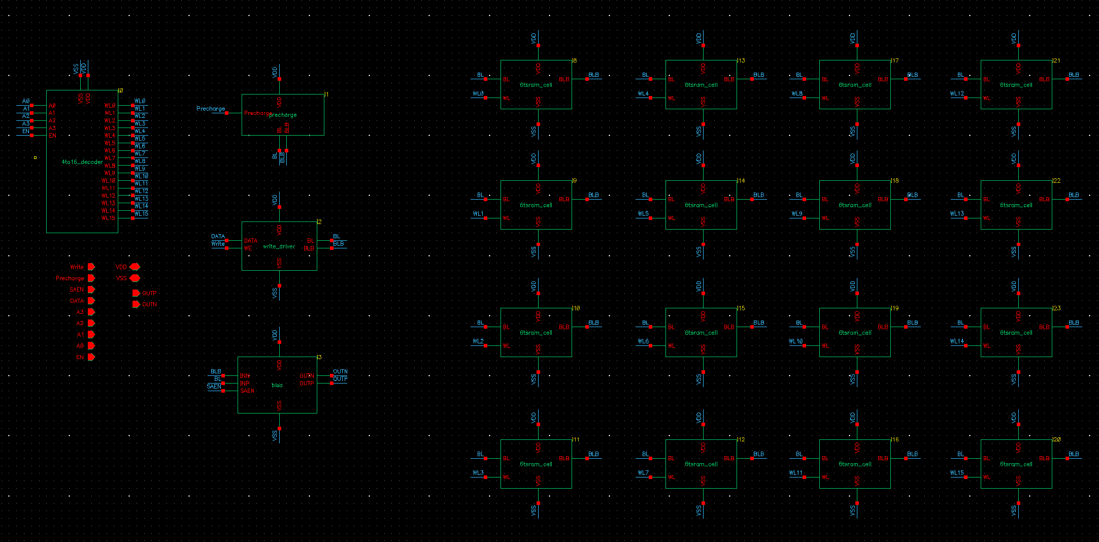
<p><img src="/images/2026-06-21/sram_1col_s.png" alt="Fig.15 : SRAM Column Schematic" /></p>

<p>Fig.15 : SRAM Column Schematic</p>

<p>The SRAM column circuit shown above was designed.</p>

<h2 id="functionality-verification-1">Functionality Verification</h2>

<h3 id="write-functionalify-verification-write-0101--">Write functionalify verification (write 0→1→0→1 .. )</h3>

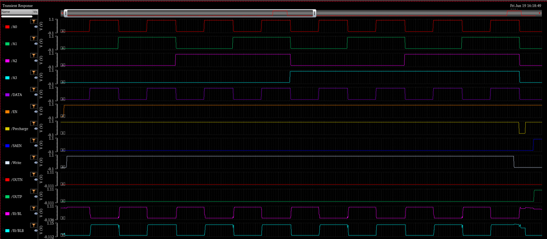
<p><img src="/images/2026-06-21/col_w0-1.png" alt="Fig.19 : SRAM Column WRITE" />
<img src="/images/2026-06-21/col_w0-2.png" alt="Fig.20 : SRAM Column WRITE" />
<img src="/images/2026-06-21/col_w0-3.png" alt="Fig.21 : SRAM Column WRITE" /></p>

<p>Fig.19-21 : SRAM Column WRITE</p>

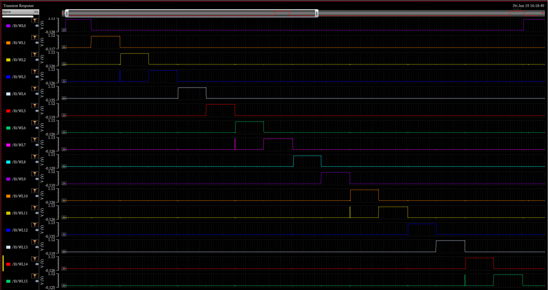
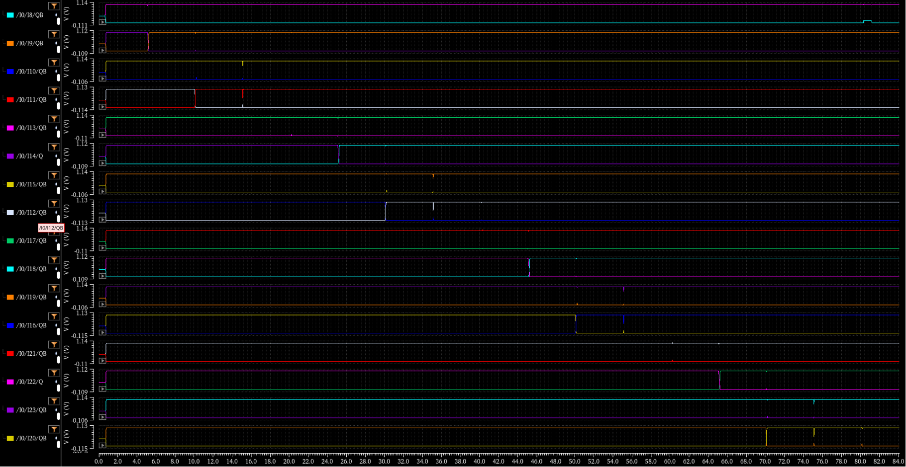
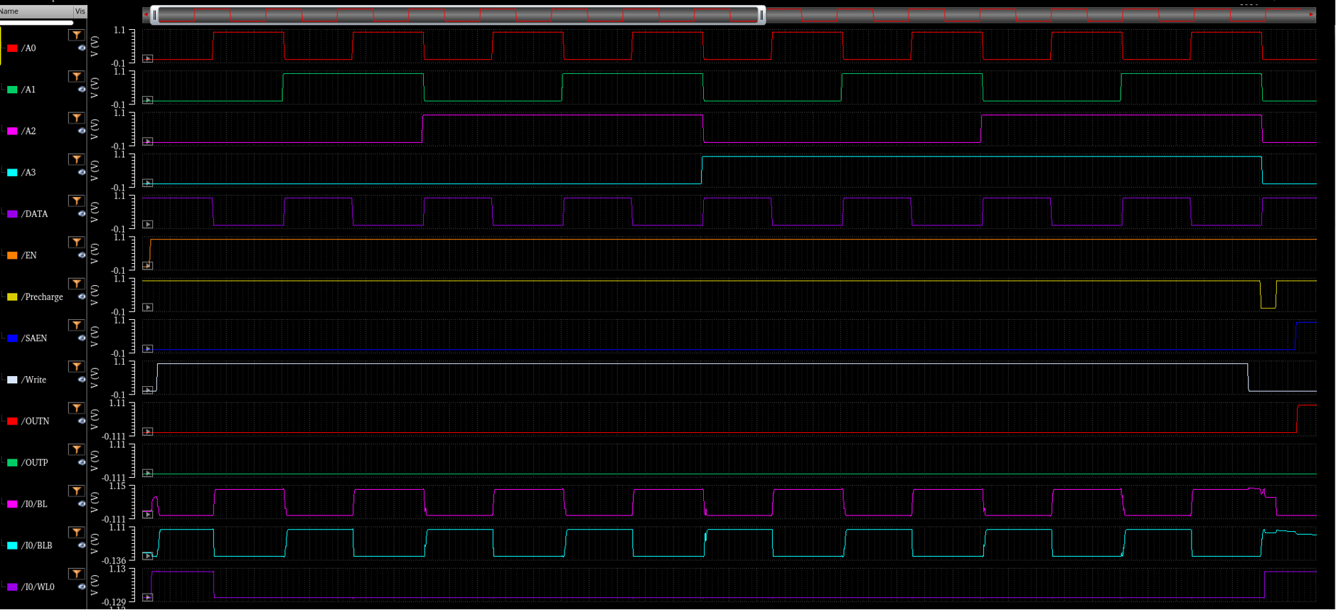
<p>The column write operation was verified using the three transient simulation results shown above.</p>

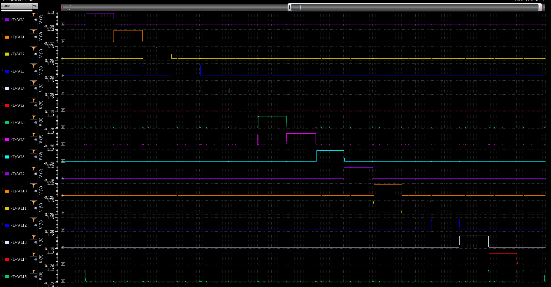
<p>In the first waveform, the outputs of the 4-to-16 decoder (WL0–WL15) are monitored. As the address inputs A3, A2, A1, A0 change sequentially, only one wordline is asserted at a time, confirming correct row selection during the write operation.</p>

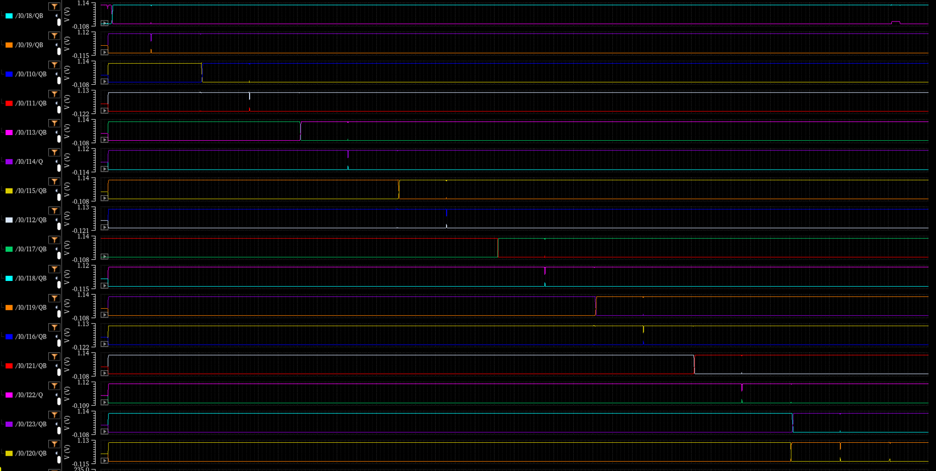
<p>The second waveform shows the internal storage nodes (Q and QB) of the SRAM cells in the selected column. Whenever a wordline is activated and the write driver applies the input data to BL and BLB, the corresponding SRAM cell changes its stored value. The complementary behavior of Q and QB confirms that the selected cell is successfully written while the unselected cells retain their previous states.</p>

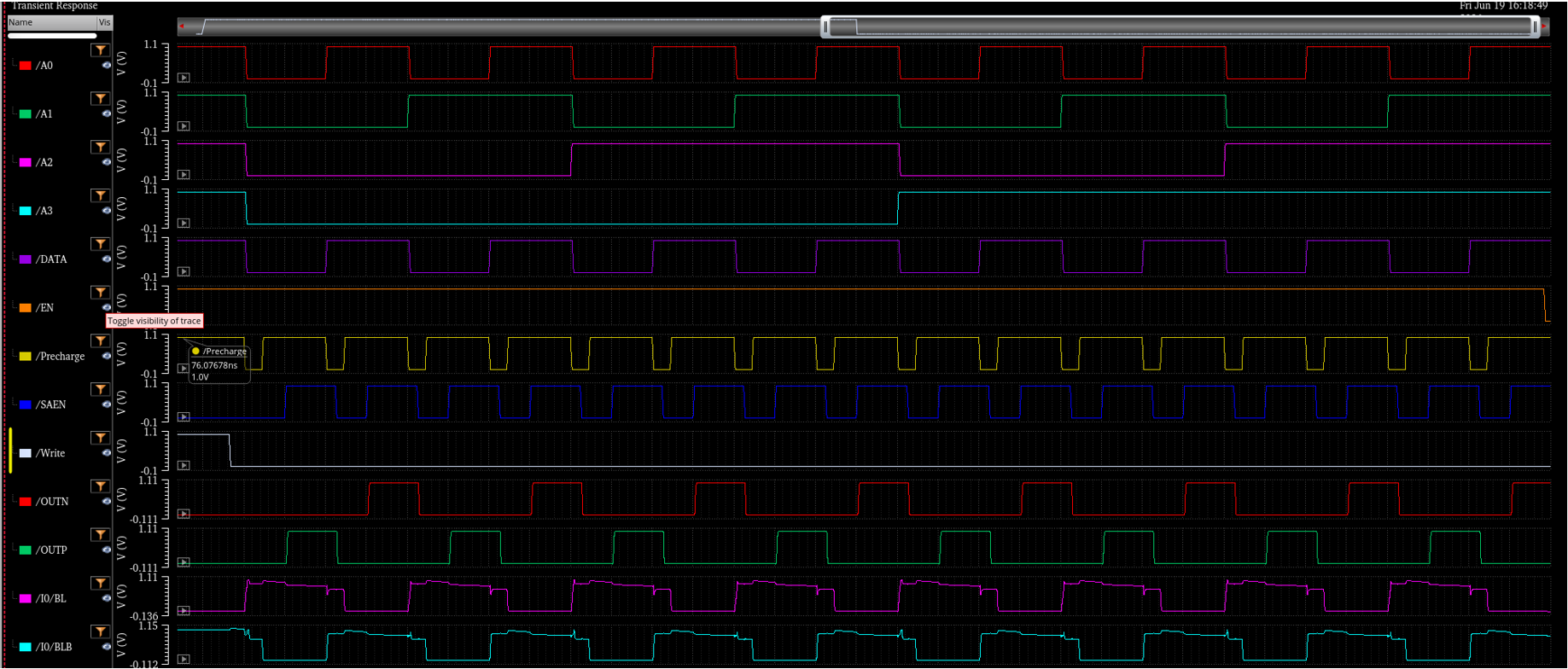
<p>The third waveform shows the address signals, DATA input, control signals, bitline voltages (BL and BLB), and sense amplifier outputs. During each write cycle, BL and BLB are driven to complementary values according to DATA by the write driver. The selected SRAM cell captures the new value through the activated wordline. The bitline transitions match the intended DATA pattern, demonstrating that the write driver, decoder, and SRAM cell operate correctly together.</p>

<p>Therefore, the three simulation results verify that the column can correctly select a target row, drive the bitlines with the desired data, and successfully store the new value in the selected SRAM cell during write operations.</p>

<h3 id="write-functionalify-verification-write-1010--">Write functionalify verification (write 1→0→1→0 .. )</h3>

<p><img src="/images/2026-06-21/col_w1-1.png" alt="Fig.16 : SRAM Column WRITE" />
<img src="/images/2026-06-21/col_w1-2.png" alt="Fig.17 : SRAM Column WRITE" />
<img src="/images/2026-06-21/col_w1-3.png" alt="Fig.18 : SRAM Column WRITE" /></p>

<p>Fig.16-18 : SRAM Column WRITE</p>

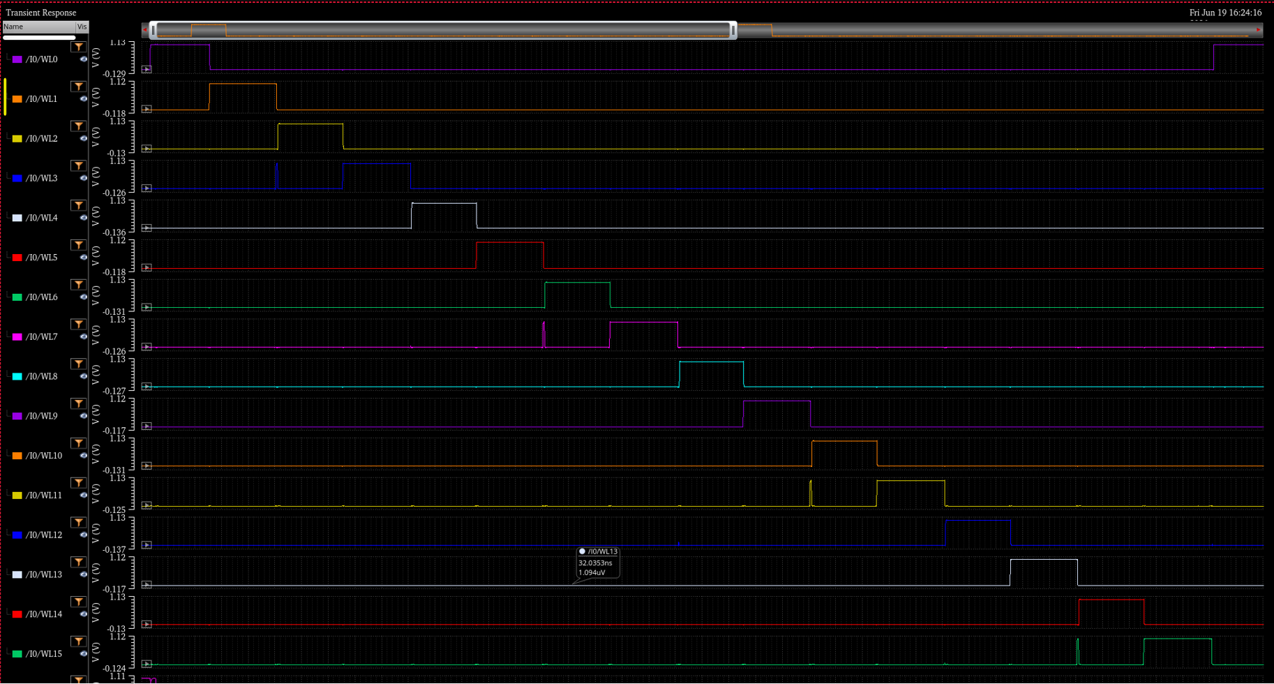
<p>The write operation was verified using the three waveforms shown above. The decoder waveform confirms that only one wordline (WL0–WL15) is activated at a time according to the address inputs. The BL and BLB waveforms show complementary bitline voltages driven by the write driver based on the DATA input. Finally, the Q and QB waveforms demonstrate that the selected SRAM cell successfully stores the written value while maintaining complementary logic states. These results confirm correct operation of the decoder, write driver, and SRAM cells during column write operations.</p>

<h3 id="read-functionality-verification">Read Functionality Verification</h3>

<p><img src="/images/2026-06-21/col_read1.png" alt="Fig.22 : SRAM Column READ" />
<img src="/images/2026-06-21/col_read2.png" alt="Fig.23 : SRAM Column READ" /></p>

<p>Fig.22-23 : SRAM Column READ</p>

<p>The read operation was verified using the waveforms shown above. The decoder outputs confirm that only one wordline (WL0–WL15) is activated at a time according to the address inputs. During each read cycle, the selected SRAM cell creates a small voltage difference between BL and BLB after precharge. When SAEN is asserted, the BLSA senses this differential voltage and amplifies it to full-swing outputs (OUTP and OUTN). The output waveforms correctly correspond to the data stored in the selected SRAM cells, confirming successful read operation of the SRAM array.</p>

<h1 id="3-16x16-sram-array-design">3. 16x16 SRAM Array Design</h1>

<p><img src="/images/2026-06-21/array.png" alt="Fig.24 : SRAM Array" /></p>

<p>Fig.24 : SRAM Array</p>

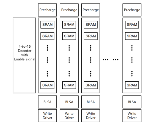
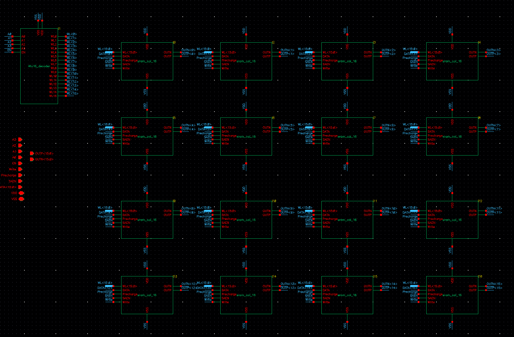
<p>This figure illustrates the overall architecture of the 16×16 SRAM array. A single 4-to-16 decoder is shared across all columns to generate the wordlines, while each column contains 16 SRAM cells connected to a dedicated precharge circuit, write driver, and BLSA. The array was designed by replicating the single-column SRAM structure sixteen times, enabling storage and access of 16-bit words in parallel.</p>

<h2 id="schematic-1">Schematic</h2>

<p><img src="/images/2026-06-21/array_s.png" alt="Fig.25 : SRAM Array Schematic" /></p>

<p>Fig.25 : SRAM Array Schematic</p>

<p>The complete 16×16 SRAM array schematic was implemented as shown above. A single 4-to-16 decoder generates the wordline signals shared by all columns, while sixteen identical SRAM columns are instantiated in parallel. Each column contains a 16-cell SRAM array, a precharge circuit, a write driver, and a BLSA, enabling parallel storage and access of 16-bit data.</p>

<h2 id="functionality-verification-2">Functionality Verification</h2>

<p><img src="/images/2026-06-21/array1.png" alt="Fig.26 : SRAM Array Verification" />
<img src="/images/2026-06-21/array2.png" alt="Fig.27 : SRAM Array Verification" />
<img src="/images/2026-06-21/array3.png" alt="Fig.28 : SRAM Array Verification" /></p>

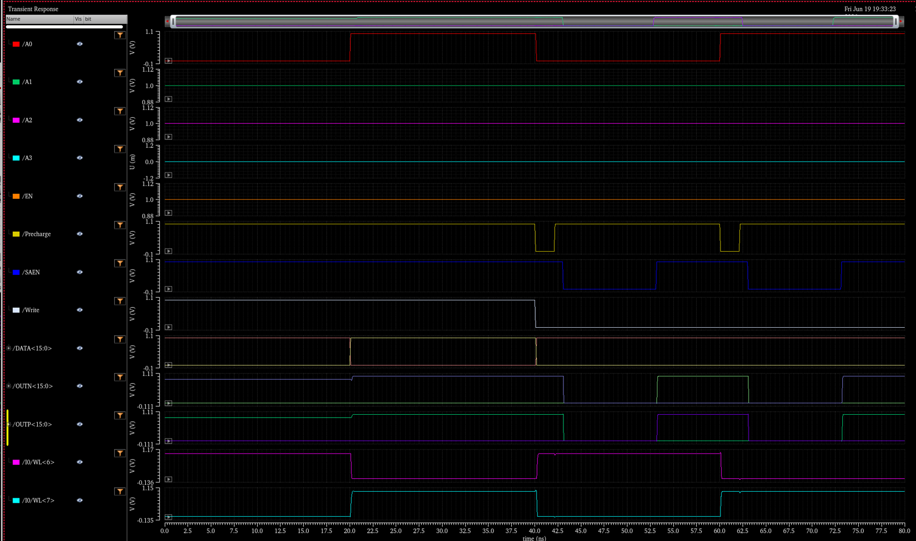
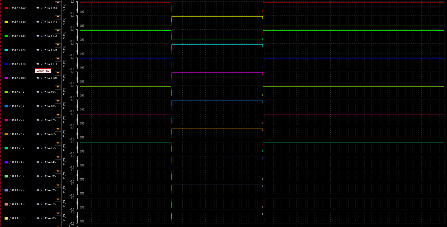
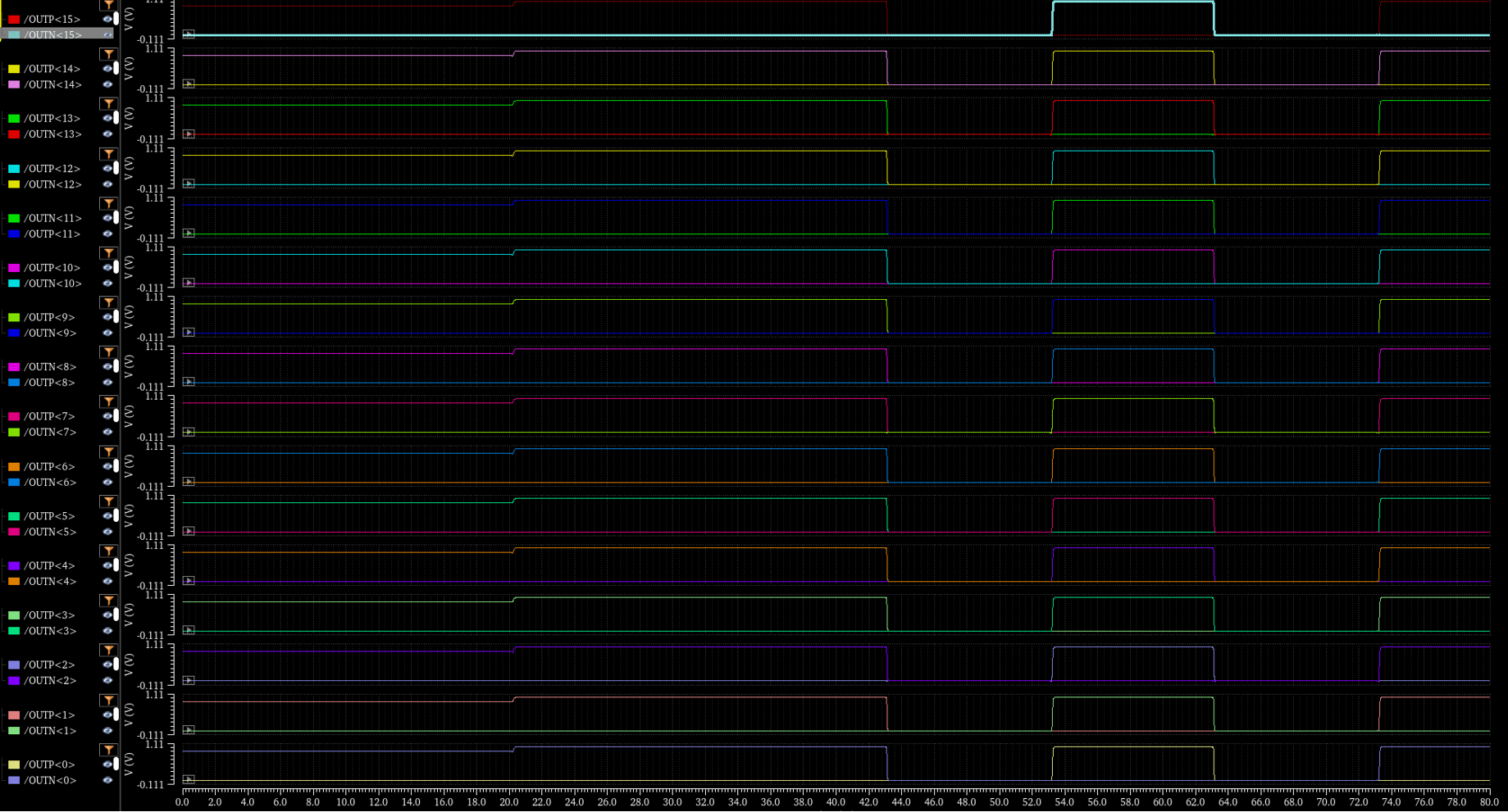
<p>Fig.26-28 : SRAM Array READ &amp; WRITE Verification</p>

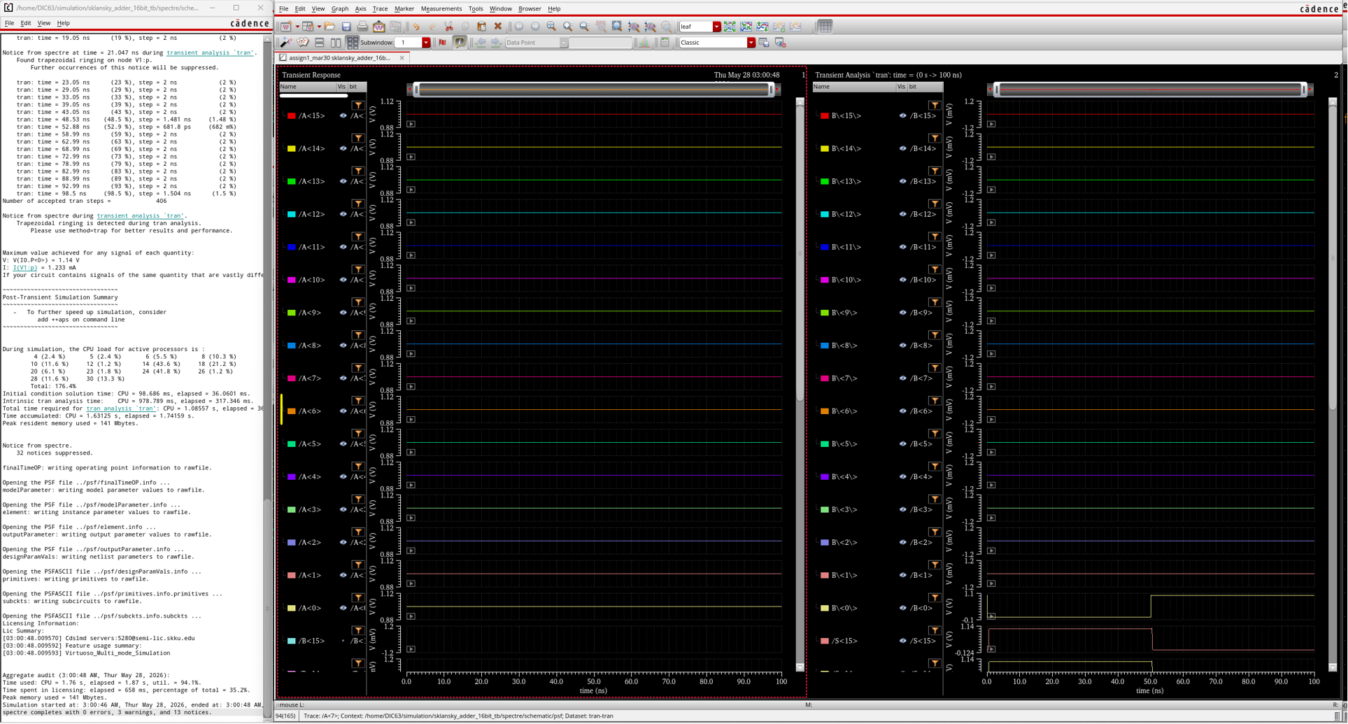
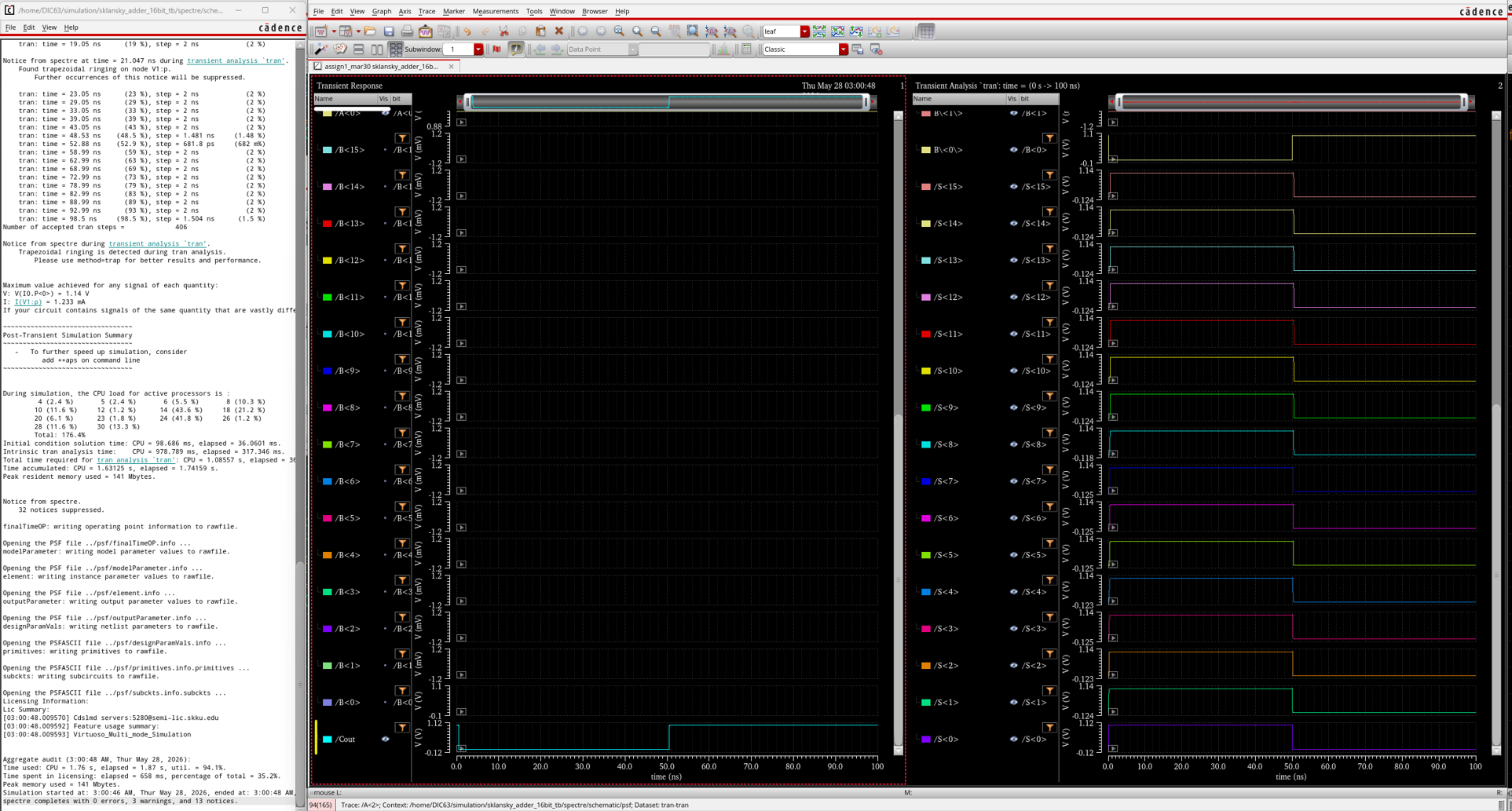
<p>To verify the functionality of the proposed 16×16 SRAM array, two rows, WL6 and WL7, were selected for write and read operations. First, the data pattern 1010101010101010 (0xAAAA) was written into WL6, followed by the complementary pattern 0101010101010101 (0x5555) written into WL7. During the write cycles, the selected wordline was activated and the write driver forced the bitlines according to the input data, causing the corresponding SRAM cells to update their stored values. As a result, WL6 and WL7 successfully stored different 16-bit data patterns.</p>

<p>For the read operation, the bitlines were precharged to VDD, after which the selected wordline generated a small voltage difference between BL and BLB depending on the stored data. When the SAEN signal was asserted, the BLSA amplified this differential voltage and produced full-swing output signals. The read results matched the data previously written into WL6 and WL7, confirming successful data storage and retrieval. These results verify the correct operation of the decoder, write driver, precharge circuit, SRAM cell array, and BLSA as an integrated 16×16 SRAM array.</p>

<h1 id="4-layout">4. Layout</h1>

<h2 id="sram-cell">SRAM Cell</h2>

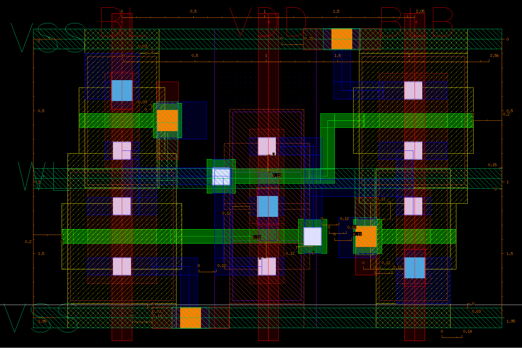
<p><img src="/images/2026-06-21/SRAM_cell_l.png" alt="Fig.29 : SRAM Cell Layout" /></p>

<p>Fig.29 : SRAM Cell Layout</p>

<p>The designed SRAM cell occupies an area of 2.05μm×1.95μm, resulting in a total cell area of 3.9975μm2.</p>

<h2 id="body-tap-cell">Body Tap Cell</h2>

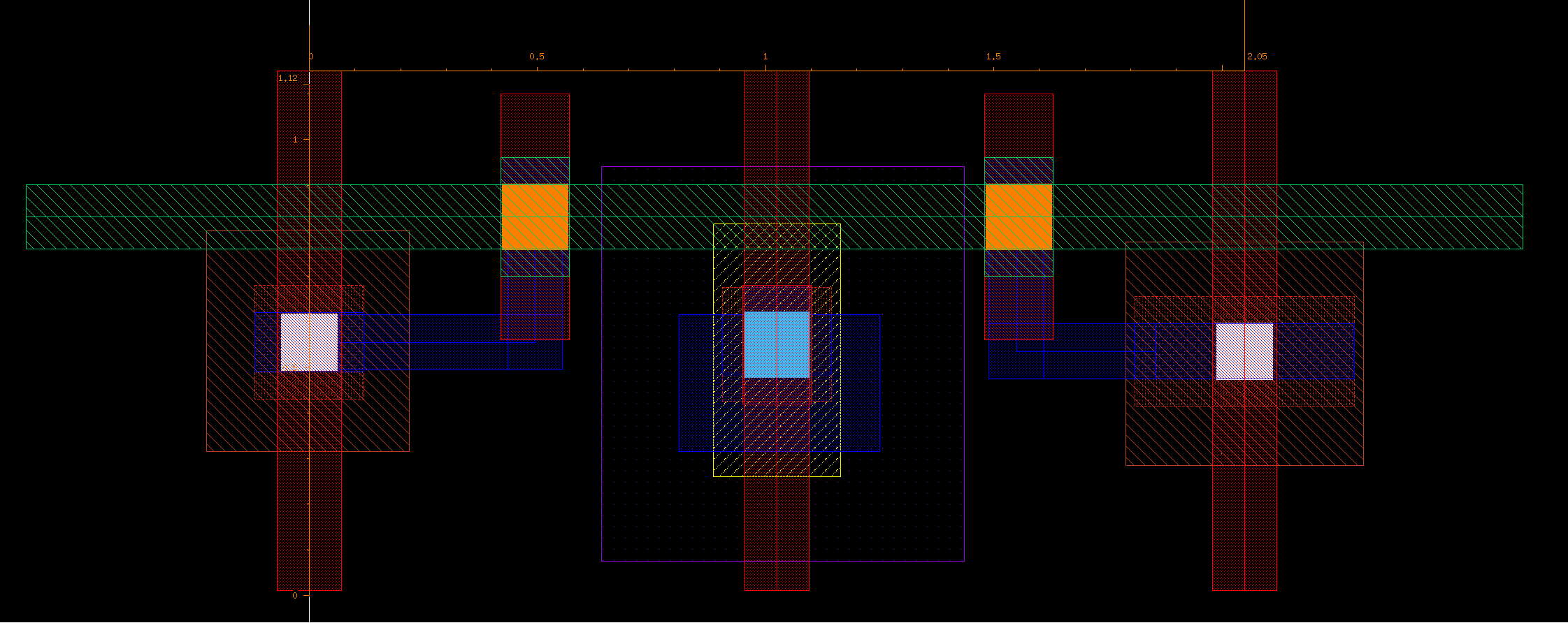
<p><img src="/images/2026-06-21/body_tap_cell.png" alt="Fig.30 : Body Tap Cell Layout" /></p>

<p>Fig.30 : Body Tap Cell Layout</p>

<p>This figure shows the layout of the body tap cell used in the SRAM array. The body tap cell provides a direct connection between the transistor bodies and the power rails (VDD and VSS), ensuring proper body biasing and preventing latch-up. In the overall layout, body tap cells are inserted periodically to maintain substrate and well potentials.</p>

<h2 id="4-to-16-decoder">4-to-16 Decoder</h2>

<p><img src="/images/2026-06-21/2-to-4-decoder_l.png" alt="Fig.31 : 2-to-4 decoder Layout" /></p>

<p>Fig.31 : 2-to-4 decoder Layout</p>

<p>This figure shows the layout of 2-to-4 decoder.</p>

<p><img src="/images/2026-06-21/4-to-16-decoder_l.png" alt="Fig.32 : 4-to-16 decoder Layout" /></p>

<p>Fig.32 : 4-to-16 decoder Layout</p>

<p>4-to-16 decoder was designed, based on the 2-to-4 decoder layout.</p>

<h2 id="blsa">BLSA</h2>

<p><img src="/images/2026-06-21/blsa_l.png" alt="Fig.33 : BLSA Layout" /></p>

<p>Fig.33 : BLSA Layout</p>

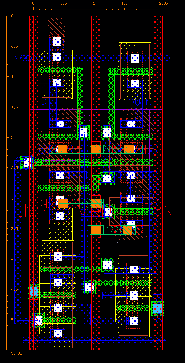
<p>This figure shows the layout design of BLSA. 
The width of the designed layout is identical to that of SRAM cell.</p>

<h2 id="write-driver">Write Driver</h2>

<p><img src="/images/2026-06-21/write_driver_l.png" alt="Fig.34 : Write Driver Layout" /></p>

<p>Fig.34 : Write Driver Layout</p>

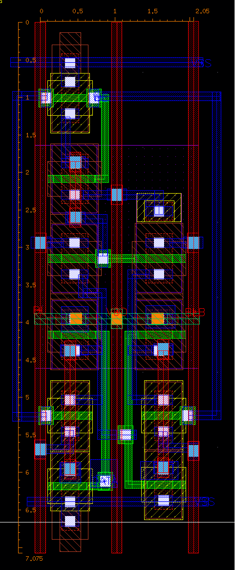
<p>This figure shows the layout design of write driver. 
The width of the designed layout is identical to that of SRAM cell.</p>

<h2 id="precharge">Precharge</h2>

<p><img src="/images/2026-06-21/precharge_l.png" alt="Fig.35 : Precharge Layout" /></p>

<p>Fig.35 : Precharge Layout</p>

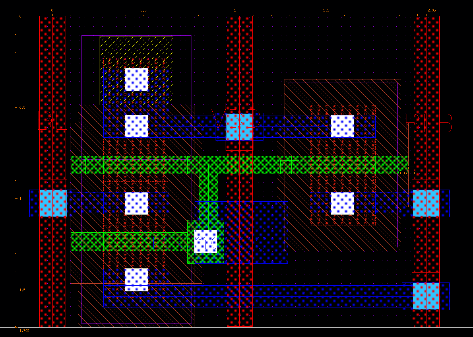
<p>This figure shows the layout design of precharge circuit. 
The width of the designed layout is identical to that of SRAM cell.</p>

<h2 id="1-column-with-16bit-sram">1 column with 16bit SRAM</h2>

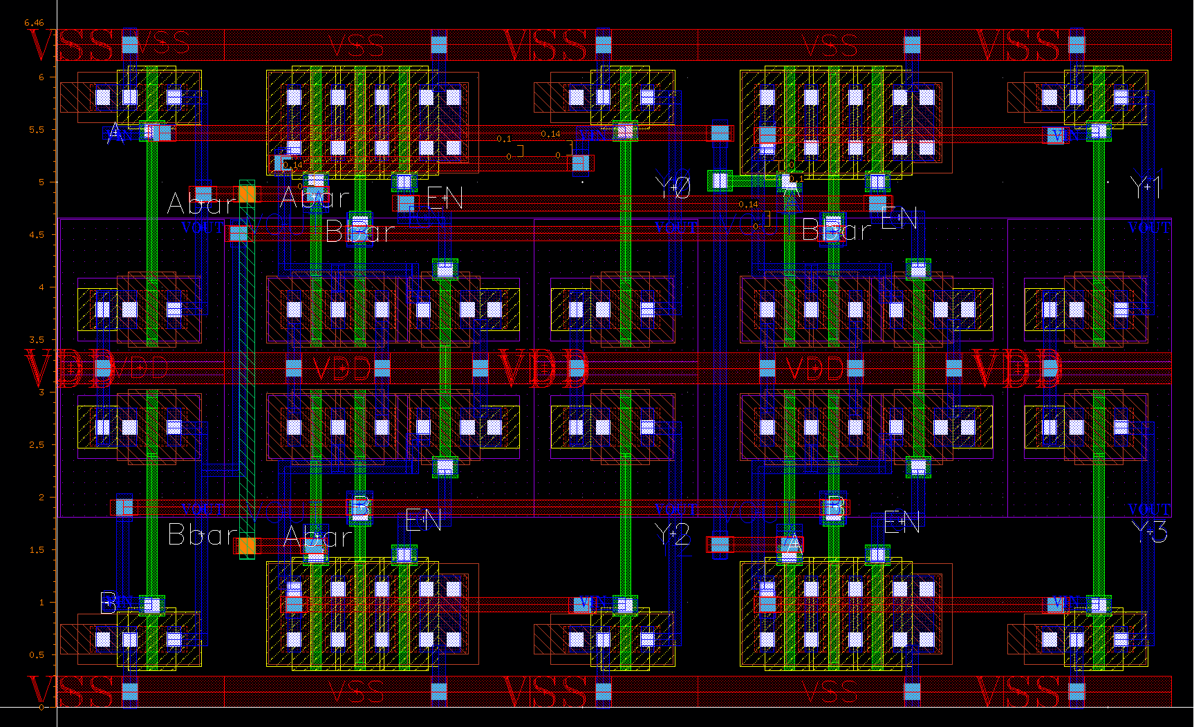
<p><img src="/images/2026-06-21/col_l.png" alt="Fig.36 : 1 Column with 16bit SRAM Layout" /></p>

<p>Fig.36 : 1 Column with 16bit SRAM Layout</p>

<p>This figure shows the layout design of SRAM column. 
For one column, the body tap cells were inserted at the top, in the middle, and at the bottom 
to prevent latch-up.</p>

<p><img src="/images/2026-06-21/col_peri_l.png" alt="Fig.37 : 1 Column with Peripheral Circuits Layout" /></p>

<p>Fig.37 : 1 Column with Peripheral Circuits Layout</p>

<p>This figure shows the layout design of SRAM 1 column, with peripheral circuits such as precharge, BLSA and write driver.</p>

<h2 id="16x16-sram-array">16x16 SRAM Array</h2>

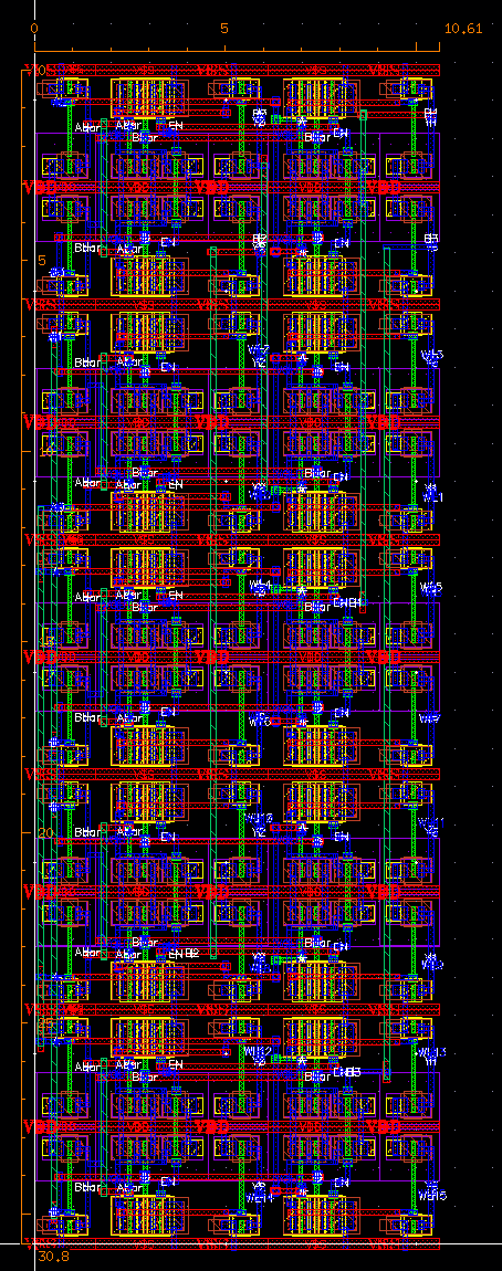
<p><img src="/images/2026-06-21/total_layout.png" alt="Fig.38 : SRAM array Layout" /></p>

<p>Fig.38 : SRAM array Layout</p>

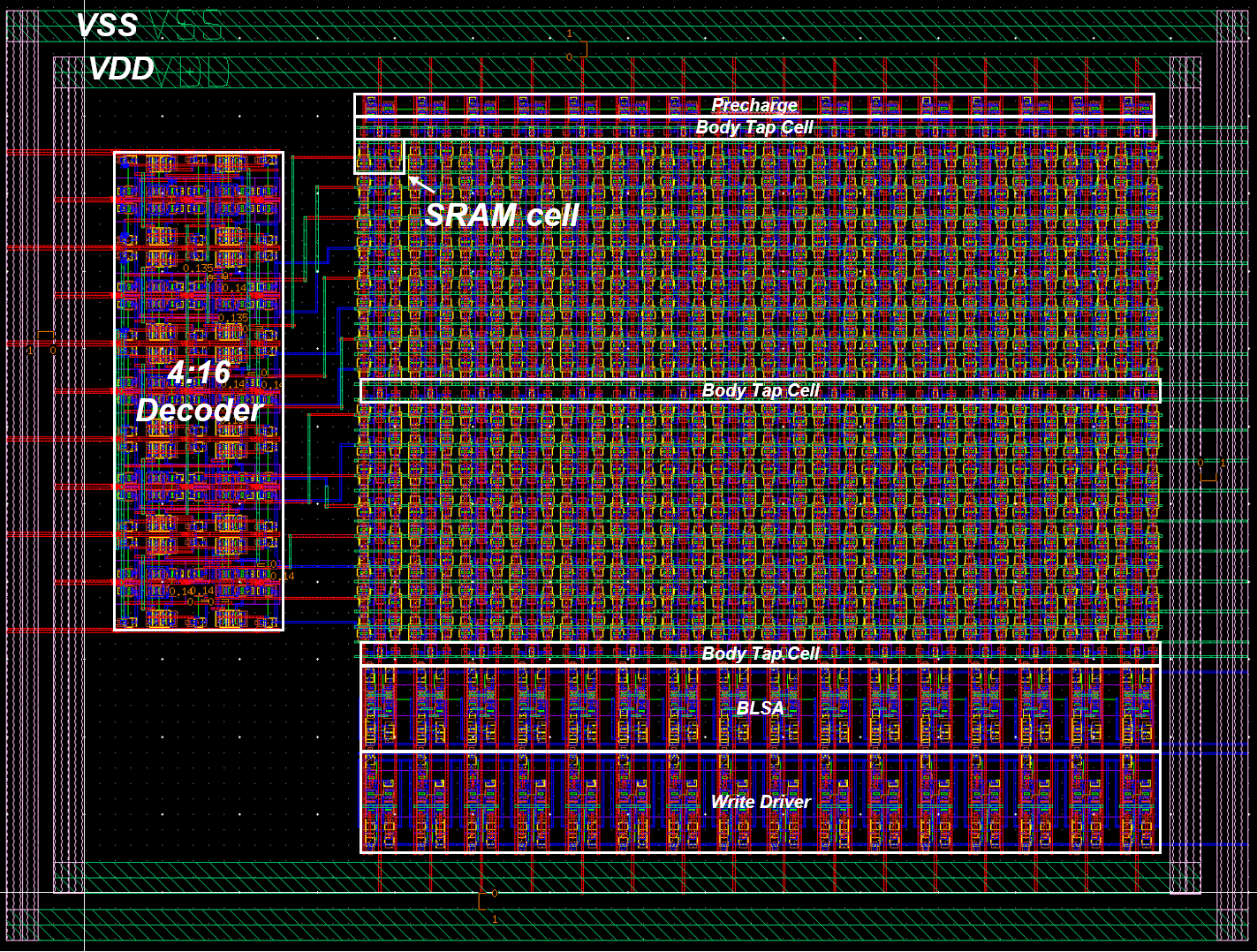
<p>The final layout implementation of the 16×16 SRAM array, including the decoder, SRAM cells, precharge circuits, write drivers, BLSAs, and body tap cells, is shown above.</p>]]></content><author><name>Seoyoon Chae</name><email>sychaeee@g.skku.edu</email></author><summary type="html"><![CDATA[This is the report submitted to Digital Integrated Circuit Design course (2026 Spring semester SSE3021, SKKU).]]></summary></entry><entry><title type="html">[SSE3021 Digital Integrated Circuit Design] Schematic and Layout Design of 16bit Sklansky Adder</title><link href="https://chae-sy.github.io/Sklansky-Adder/" rel="alternate" type="text/html" title="[SSE3021 Digital Integrated Circuit Design] Schematic and Layout Design of 16bit Sklansky Adder" /><published>2026-06-20T00:00:00+00:00</published><updated>2026-06-20T00:00:00+00:00</updated><id>https://chae-sy.github.io/Sklansky-Adder</id><content type="html" xml:base="https://chae-sy.github.io/Sklansky-Adder/"><![CDATA[<p>This is the report submitted to Digital Integrated Circuit Design course (2026 Spring semester SSE3021, SKKU).</p>

<h1 id="1-introduction-to-sklansky-adder">1. Introduction to Sklansky Adder</h1>

<h2 id="pgd-notation">PGD Notation</h2>

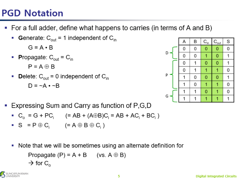
<p><img src="/images/2026-06-20/image1.png" alt="Fig.1 : PGD Notation" /></p>

<p>Fig.1 : PGD Notation</p>

<p>PGD (Propagate, Generate, Delete) notation is a method used to describe carry behavior in a full adder based only on the input bits A and B.</p>

<p>Generate (\(\text{G} = \text{A} \cdot \text{B}\)): The adder generates a carry regardless of the input carry, so \(\text{C}_{out}=1\).
Propagate (\(\text{P} = \text{A} \oplus \text{B}\)): The input carry is propagated to the output, so \(\text{C}_{out}=\text{C}_{in}\).</p>

<p>Delete (\(\text{D} = \overline{A}\cdot\overline{B}\)): The carry is deleted regardless of the input carry, so \(\text{C}_{out}=0\).</p>

<p>Using PGD notation, the carry and sum outputs can be expressed as:</p>

\[\text{C}_{out}=\text{G}+\text{P} \cdot \text{C}_{in}\]

\[\text{S}=\text{P} \oplus \text{C}_{in}\]

<p>This notation simplifies carry analysis and is widely used in high-speed adder designs such as carry-lookahead and parallel-prefix adders.</p>

<h2 id="look-ahaed-adder">Look Ahaed Adder</h2>

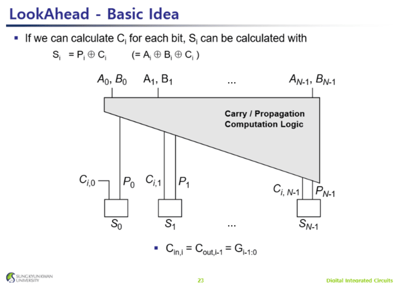
<p><img src="/images/2026-06-20/image2.png" alt="Fig.2 : Look Ahaed Adder" /></p>

<p>Fig.2 : Look Ahaed Adder</p>

<p>The basic idea of carry lookahead logic. Instead of waiting for the carry signal to ripple through each bit one by one, the circuit computes all carry signals \(\text{C}_{i}\) in parallel using the propagate (P) and generate (G) signals. Once the carry for each bit is available, the sum can be calculated as</p>

<p>\(\text{S}_{i} = \text{P}_{i} \oplus \text{C}_{i} = \text{A}_{i}\oplus \text{B}_{i} \oplus\text{C}_{i}\).</p>

<p>The carry/propagation computation block receives all input bits (\(\text{A}_{i}, \text{B}_{i}\)) and quickly determines the carry for every stage. This parallel carry computation significantly reduces delay compared to a ripple-carry adder, making carry lookahead adders much faster for large bit-width additions.</p>

<h2 id="black-cell-gray-cell-and-buffer">Black Cell, Gray Cell and Buffer</h2>

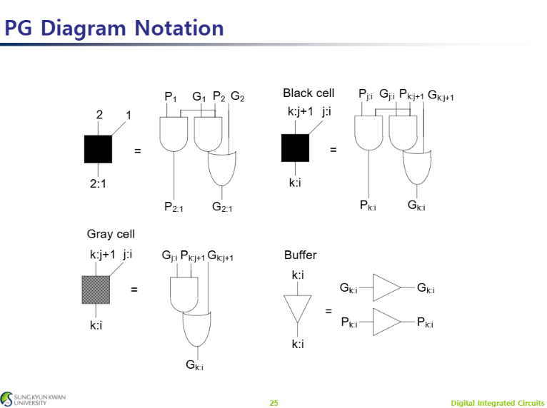
<p><img src="/images/2026-06-20/image3.png" alt="Fig.3 : Black cell, Gray cell and Buffer" /></p>

<p>Fig.3 : Black cell, Gray cell and Buffer</p>

<p>There are fundamental building blocks used in parallel-prefix adders, such as the Kogge–Stone adder. These cells combine propagate (P) and generate (G) signals to efficiently compute carry information across multiple bit positions.</p>

<p><strong>Black Cell</strong>: Combines two PG pairs and produces both a new propagate and a new generate signal:</p>

\[\text{P}_{k:i} = \text{P}_{j:i} \cdot \text{P}_{k:j+1}\]

\[\text{G}_{k:i}=\text{G}_{k:j+1}+\text{P}_{k:j+1} \cdot \text{G}_{j:i}\]

<p>Since it outputs both P and G, it is used in intermediate stages of the prefix network.</p>

<p><strong>Gray Cell</strong>: Computes only the generate signal:</p>

\[\text{G}_{k:i} = \text{G}_{k:j+1} + \text{P}_{k:j+1} \cdot \text{G}_{j:i}\]

<p>Because only the carry information is needed at the final stage, the propagate output is omitted, reducing hardware complexity.</p>

<p><strong>Buffer</strong>: Simply forwards the existing P and G signals without modification. It is used to balance timing and maintain a regular network structure.</p>

<p>By repeatedly combining PG signals with black and gray cells, a parallel-prefix adder can calculate carries for all bits in parallel, achieving much lower delay than a ripple-carry adder.</p>

<h2 id="sklansky-adder">Sklansky Adder</h2>

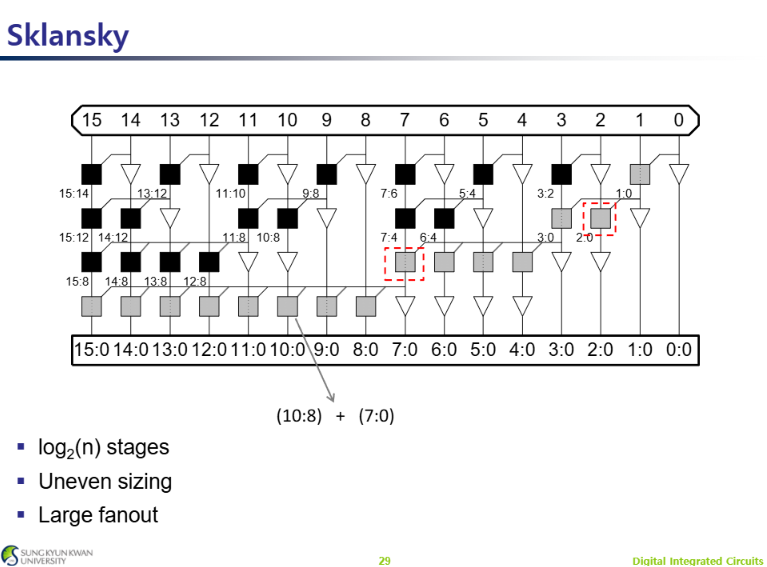
<p><img src="/images/2026-06-20/image4.png" alt="Fig.4 : Sklansky Adder" /></p>

<p>Fig.4 : Sklansky Adder</p>

<p>The structure of a 16-bit Sklansky parallel-prefix adder is as the above image, which is designed to compute carry signals with low logic depth. The network combines propagate (P) and generate (G) signals through a hierarchy of black and gray cells to determine carries for all bit positions.</p>

<p>A key advantage of the Sklansky adder is that it requires only \(\log_2(n)\) stages, allowing carry signals to be generated much faster than in a ripple-carry adder. At each stage, larger groups of bits are combined, such as (10:8) and (7:0), to form wider carry prefixes.</p>

<p>However, the Sklansky structure has some drawbacks. The distribution of logic is uneven, meaning that some nodes drive significantly more outputs than others. This results in large fanout, especially near the most significant bits, which can increase delay and power consumption in practical implementations. Despite this limitation, the Sklansky adder remains attractive because of its small logic depth and relatively low hardware complexity.</p>

<h1 id="2-basic-cell-design-for-carry-lookahead-adder">2. Basic Cell Design for Carry Lookahead Adder</h1>

<h2 id="setup-cell">Setup Cell</h2>

<p><img src="/images/2026-06-20/setup.png" alt="Fig.5 : Setup Cell" /></p>

<p>Fig.5 : Setup Cell</p>

<h2 id="carry-cell">Carry Cell</h2>

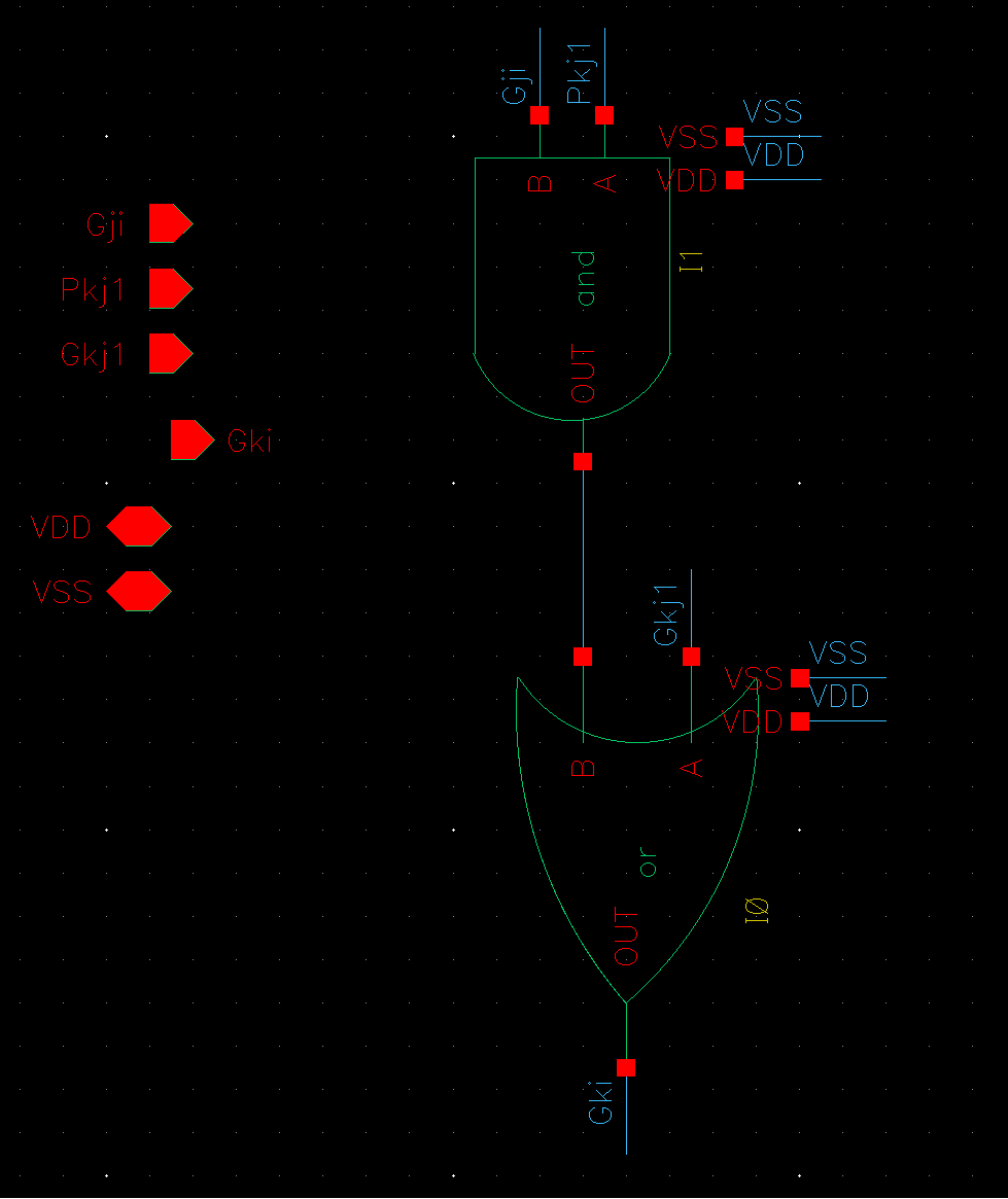
<p><img src="/images/2026-06-20/carry.png" alt="Fig.6 : Carry Cell" /></p>

<p>Fig.6 : Carry Cell</p>

<h2 id="sum-cell">Sum Cell</h2>

<p><img src="/images/2026-06-20/sum.png" alt="Fig.7 : Sum Cell" /></p>

<p>Fig.7 : Sum Cell</p>

<h2 id="black-cell">Black Cell</h2>

<p><img src="/images/2026-06-20/black.png" alt="Fig.8 : Black Cell" /></p>

<p>Fig.8 : Black Cell</p>

<h2 id="gray-cell">Gray Cell</h2>

<p><img src="/images/2026-06-20/gray.png" alt="Fig.9 : Gray Cell" /></p>

<p>Fig.9 : Gray Cell</p>

<h1 id="3-16bit-carry-lookahead-adder-design">3. 16bit Carry Lookahead Adder Design</h1>

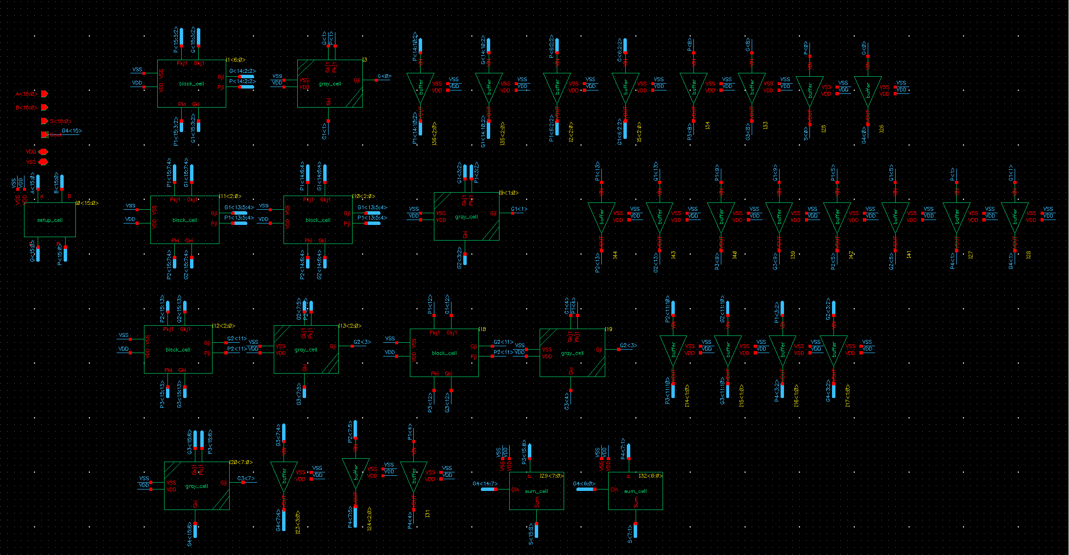
<h2 id="sklansky-adder-1">Sklansky Adder</h2>

<p><img src="/images/2026-06-20/sklansky.png" alt="Fig.10 : Sklansky Adder" /></p>

<p>Fig.10 : Sklansky Adder</p>

<h2 id="sklansky-adder-with-flip-flops">Sklansky Adder with Flip Flops</h2>

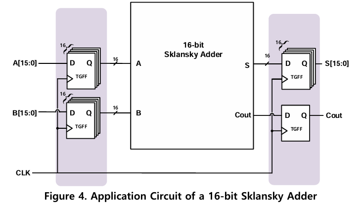
<p><img src="/images/2026-06-20/fig_sklansky_ff.png" alt="Fig.11 : Sklansky Adder with Flip Flops" /></p>

<p>Fig.11 : Sklansky Adder with Flip Flops</p>

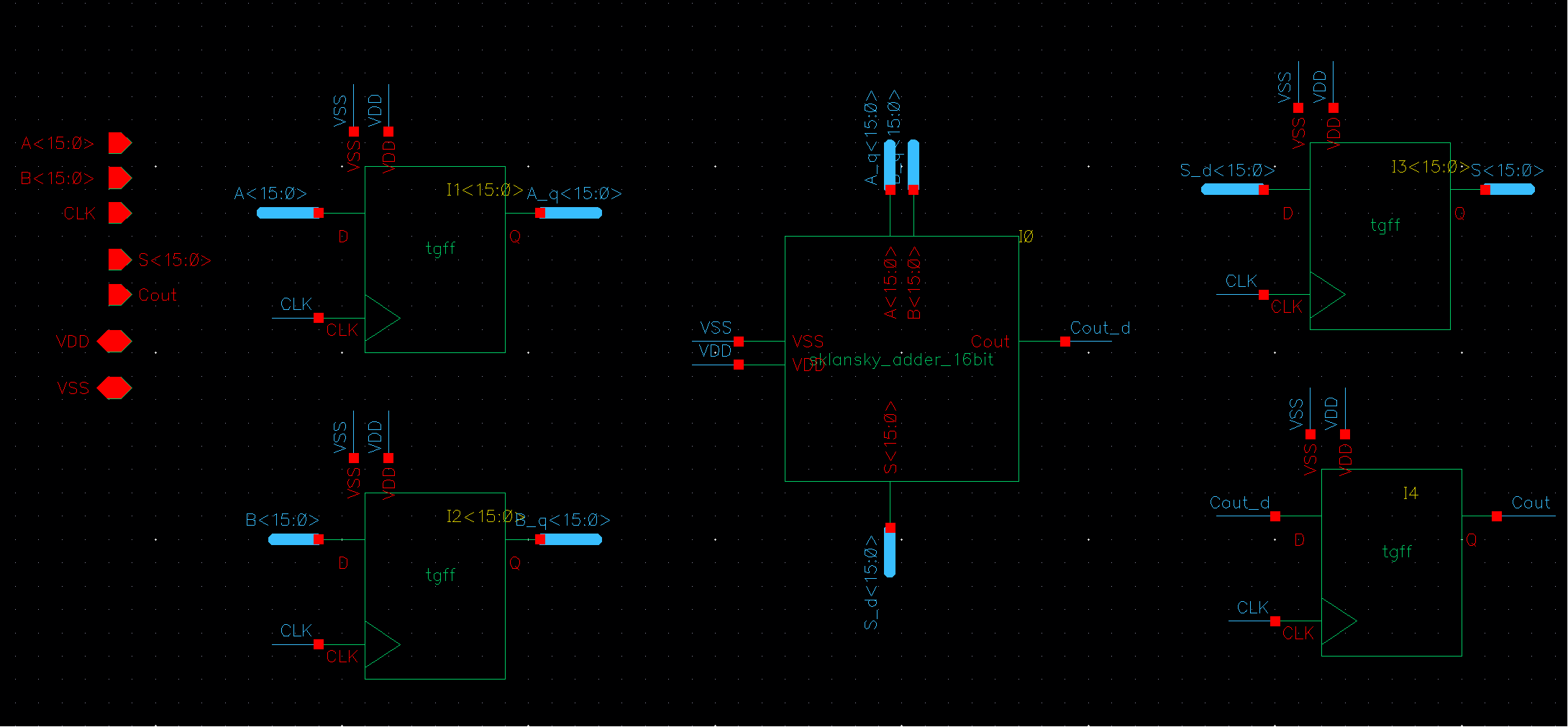
<p><img src="/images/2026-06-20/sklansky_ff.png" alt="Fig.12 : Sklansky Adder with Flip Flops Design" /></p>

<p>Fig.12 : Sklansky Adder with Flip Flops Design</p>

<p>This figure shows the application circuit used to verify the 16-bit Sklansky adder. To accurately evaluate the adder under realistic operating conditions, flip-flops (FFs) were placed at both the input and output sides of the adder.</p>

<p>The input flip-flops register the 16-bit operands A[15:0] and B[15:0] on the rising edge of the clock and provide stable inputs to the Sklansky adder. The adder then performs the addition and generates the sum S[15:0] and carry-out (Cout). The output flip-flops capture these results at the next clock edge, enabling synchronous operation and accurate timing measurements.</p>

<p>By surrounding the combinational adder with input and output registers, the circuit can be simulated and analyzed as a pipelined system, allowing the propagation delay and overall performance of the 16-bit Sklansky adder to be verified more reliably.</p>

<h2 id="functionality-verification">Functionality Verification</h2>

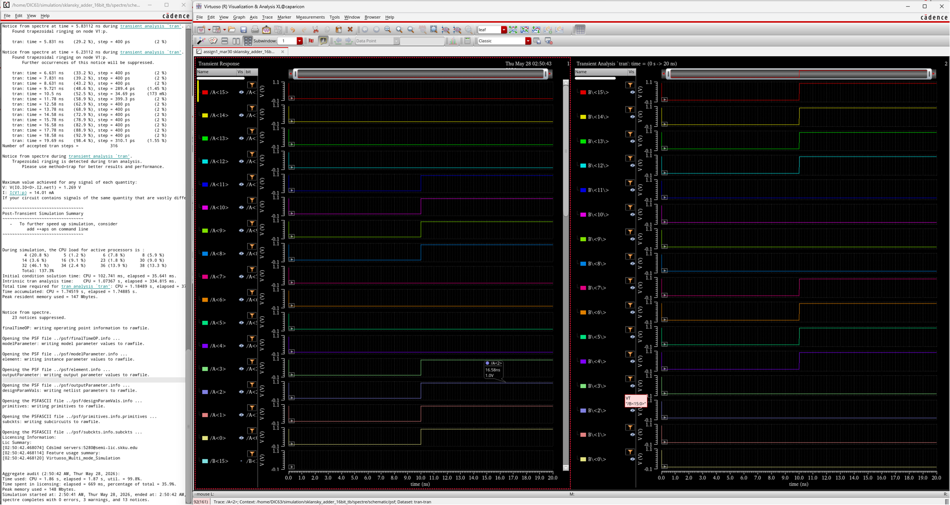
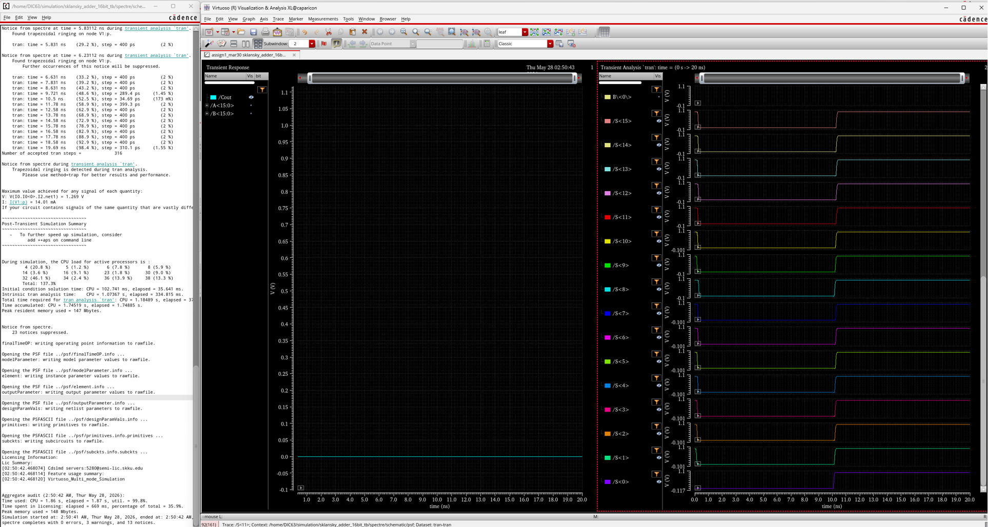
<h3 id="case-1">Case 1.</h3>

<p><img src="/images/2026-06-20/case1-1.png" alt="Fig.13 : Case 1_1" /></p>

<p><img src="/images/2026-06-20/case1-2.png" alt="Fig.14 : Case 1_2" /></p>

<p>Fig. 13-14 : Case 1</p>

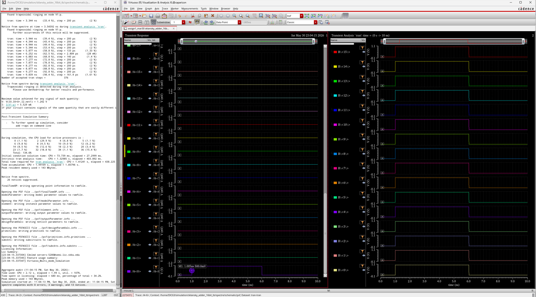
<p>A=0000_0000_0000_0000 → 0000_1111_0000_1111</p>

<p>B=0000_0000_0000_0000 → 1111_0000_1111_0000</p>

<p>S=0000_0000_0000_0000 → 1111_1111_1111_1111</p>

<p>Cout = 0</p>

<h3 id="case-2">Case 2.</h3>

<p><img src="/images/2026-06-20/case2-1.png" alt="Fig.15 : Case 2_1" /></p>

<p><img src="/images/2026-06-20/case2-2.png" alt="Fig.16 : Case 2_2" /></p>

<p>Fig. 15-16 : Case 2</p>

<p>A=1111_1111_1111_1111</p>

<p>B=0000_0000_0000_0000 → 0000_0000_0000_0001</p>

<p>S=1111_1111_1111_1111 → 0000_0000_0000_0000</p>

<p>Cout = 0 → 1</p>

<h3 id="case-3">Case 3.</h3>

<p><img src="/images/2026-06-20/case3-1.png" alt="Fig.17 : Case 3_1" /></p>

<p><img src="/images/2026-06-20/case3-2.png" alt="Fig.18 : Case 3_2" /></p>

<p>Fig. 17-18 : Case 3</p>

<p>A = 0000 0000 0000 0000 → 0000 0000 0000 0001</p>

<p>B = 0000 0000 0000 0000 → 1111 1111 1111 1111</p>

<p>S = 0000 0000 0000 0000 → 0000 0000 0000 0000</p>

<p>Cout = 0 → 1</p>

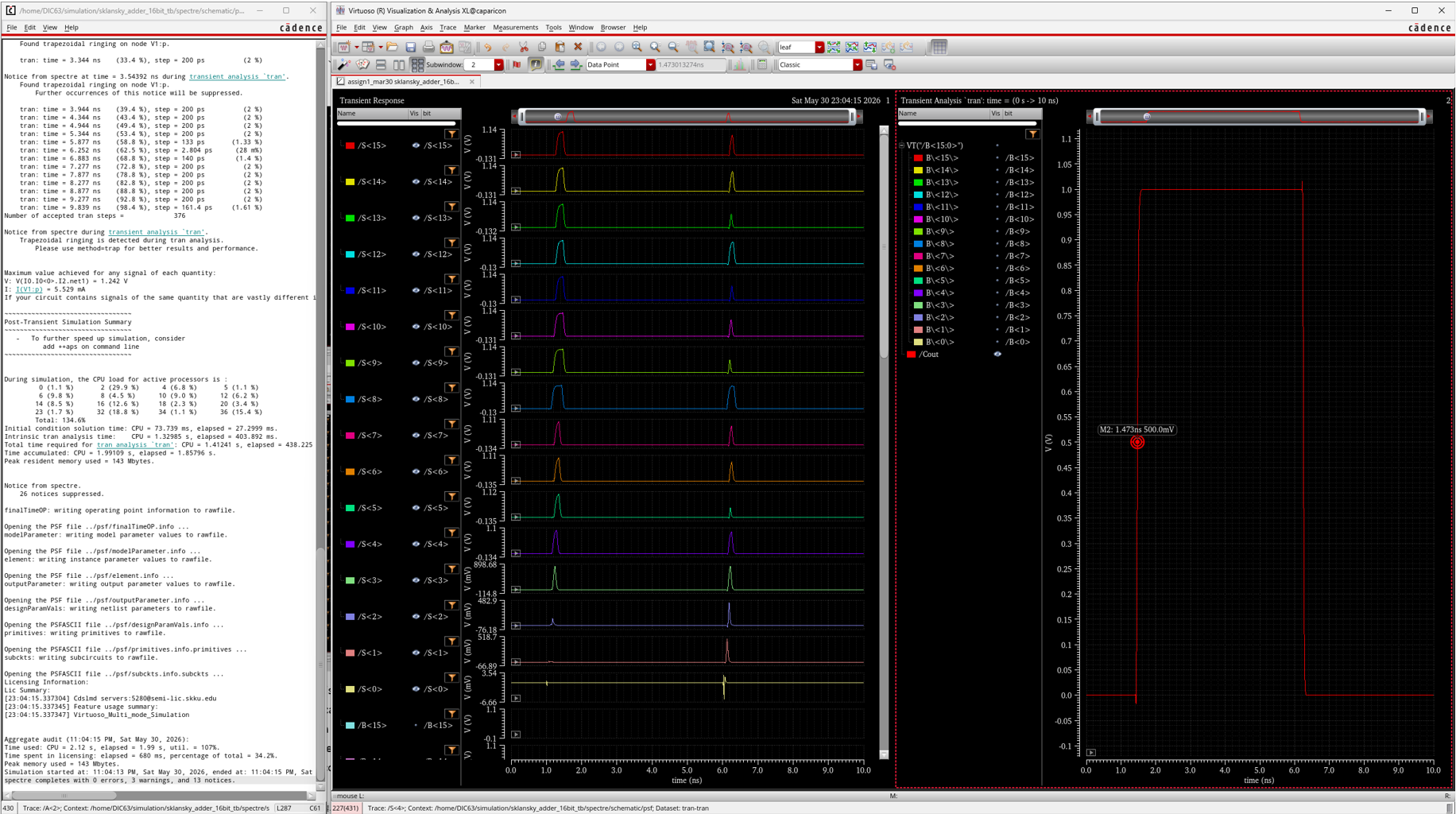
<p>Although the final sum output is zero, temporary glitches were observed on the sum bits during the input transition. This occurs because the propagate signals reach the sum XOR gates earlier than the carry signals generated through the prefix tree. As a result, the sum output temporarily changes before the correct carry arrives, and then settles to the correct final value. Therefore, these glitches are caused by unequal path delays in the combinational Sklansky adder and do not indicate a functional error.</p>

<p>This case occurs the worst case delay since it is a pattern such that a carry is generated at the least significant bit and propagated through all higher bits to the final carry-out. In this case, bit 0 generates a carry, while bits 1 through 15 are in the propagate condition. Therefore, the carry must travel through the longest prefix path of the 16-bit Sklansky adder, producing the worst-case delay at Cout.</p>

\[\text{T}_{delay, Cout}  = 1.473ns – 1.005ns = 0.468ns\]

<h1 id="4-layout-design-of-basic-cells">4. Layout Design of Basic cells</h1>

<h2 id="setup-cell-1">Setup Cell</h2>

<p><img src="/images/2026-06-20/setup_l.png" alt="Fig.19 : Setup Cell" /></p>

<p>Fig.19 : Setup Cell</p>

<h2 id="carry-cell-1">Carry Cell</h2>

<p><img src="/images/2026-06-20/carry_l.png" alt="Fig.20 : Carry Cell" /></p>

<p>Fig.20 : Carry Cell</p>

<h2 id="sum-cell-1">Sum Cell</h2>

<p><img src="/images/2026-06-20/sum_l.png" alt="Fig.21 : Sum Cell" /></p>

<p>Fig.21 : Sum Cell</p>

<h2 id="black-cell-1">Black Cell</h2>

<p><img src="/images/2026-06-20/black_l.png" alt="Fig.22 : Black Cell" /></p>

<p>Fig.22 : Black Cell</p>

<h2 id="gray-cell-1">Gray Cell</h2>

<p><img src="/images/2026-06-20/gray_l.png" alt="Fig.23 : Gray Cell" /></p>

<p>Fig.23 : Gray Cell</p>

<h2 id="tgff">TGFF</h2>

<p><img src="/images/2026-06-20/tgff.png" alt="Fig.24 : TGFF Schematic" /></p>

<p><img src="/images/2026-06-20/tgff_l.png" alt="Fig.25 : TGFF Layout" /></p>

<p>Fig.24-25 : TGFF Schematic and Layout</p>

<h1 id="5-layout-design-of-16bit-sklansky-adder">5. Layout Design of 16bit sklansky adder</h1>

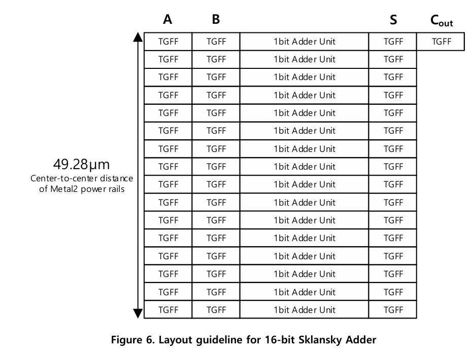
<p><img src="/images/2026-06-20/floorplan.png" alt="Fig.26: Floorplan" /></p>

<p>Fig.26 : Floorplan</p>

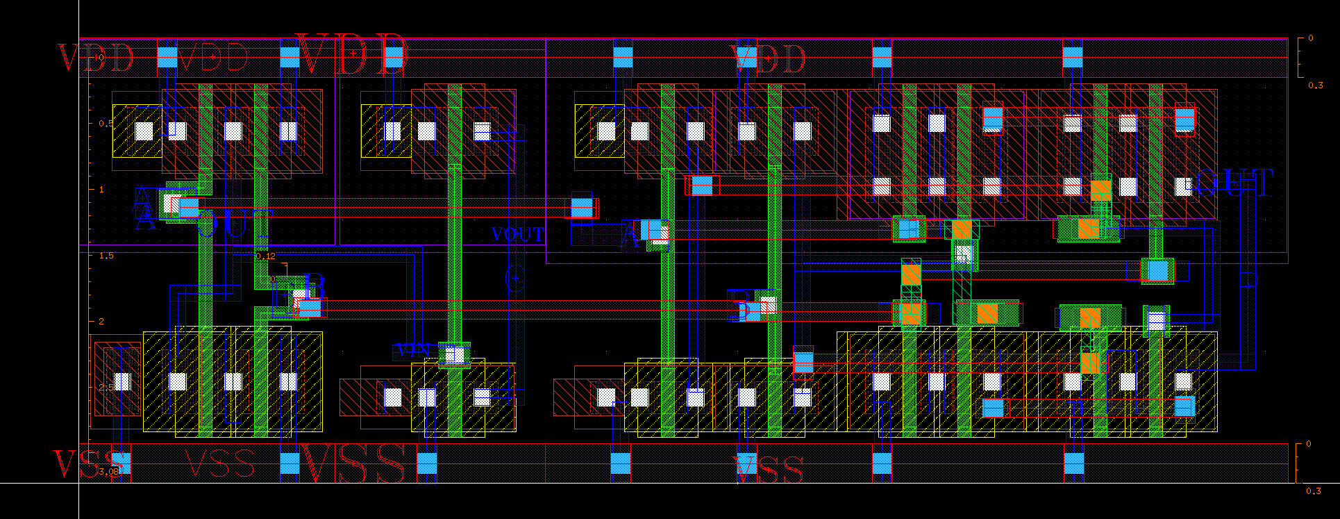
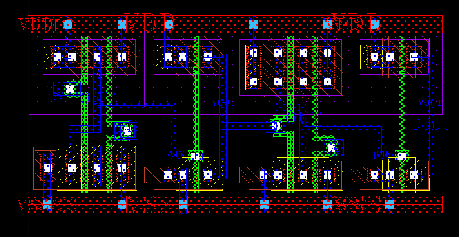
<p>This figure illustrates the floorplan of the 16-bit Sklansky adder, where 16 one-bit adder units are arranged vertically between input and output TGFFs to achieve a regular layout structure while satisfying the 49.28 μm center-to-center spacing requirement of the Metal2 power rails.</p>

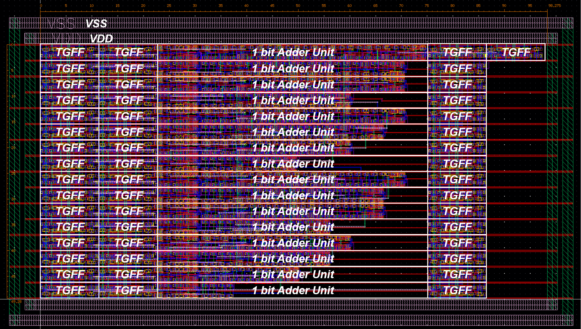
<p><img src="/images/2026-06-20/total_layout.png" alt="Fig.27: Layout" /></p>

<p>Fig.27 : Final Layout</p>

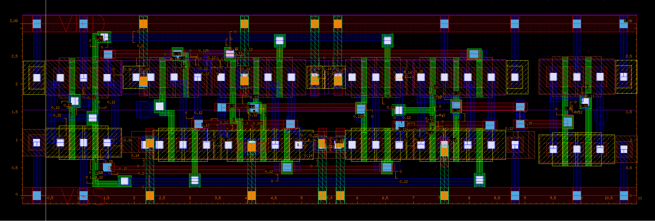
<p>This figure shows the final layout implementation of the 16-bit Sklansky adder in Cadence Virtuoso, where the TGFFs are placed on both sides of the adder core and the routing is completed while maintaining the required power rail structure and layout constraints.</p>]]></content><author><name>Seoyoon Chae</name><email>sychaeee@g.skku.edu</email></author><summary type="html"><![CDATA[This is the report submitted to Digital Integrated Circuit Design course (2026 Spring semester SSE3021, SKKU).]]></summary></entry><entry><title type="html">[Project] CUDA Matrix Multiplication Implementation and Optimization</title><link href="https://chae-sy.github.io/CUDA-MatMul/" rel="alternate" type="text/html" title="[Project] CUDA Matrix Multiplication Implementation and Optimization" /><published>2025-12-17T00:00:00+00:00</published><updated>2025-12-17T00:00:00+00:00</updated><id>https://chae-sy.github.io/CUDA-MatMul</id><content type="html" xml:base="https://chae-sy.github.io/CUDA-MatMul/"><![CDATA[<p>Implemented and optimized CUDA kernels for scaled dot-product attention, attention linear projection, and Q/K/V projection.</p>

<h1 id="1-implementation-of-scaled-dot-product-attention-using-cuda-kernels">1. Implementation of Scaled Dot-Product Attention Using CUDA Kernels</h1>

<p>The scaled dot-product attention operation was implemented on NVIDIA RTX 4060 Ti, RTX 5080, and L40S GPUs. Various optimization techniques previously applied to matrix multiplication on the Ada architecture were adapted to the attention computation.</p>

<p>The computation pipeline consisted of three kernels. The (QK^T) matrix multiplication and attention mask addition were fused into a single kernel, followed by a softmax kernel and a matrix multiplication kernel for (PV). Through this design, the entire scaled dot-product attention could be executed using only three CUDA kernels.</p>

<h2 id="11-shared-memory-tiling">1.1 Shared Memory Tiling</h2>
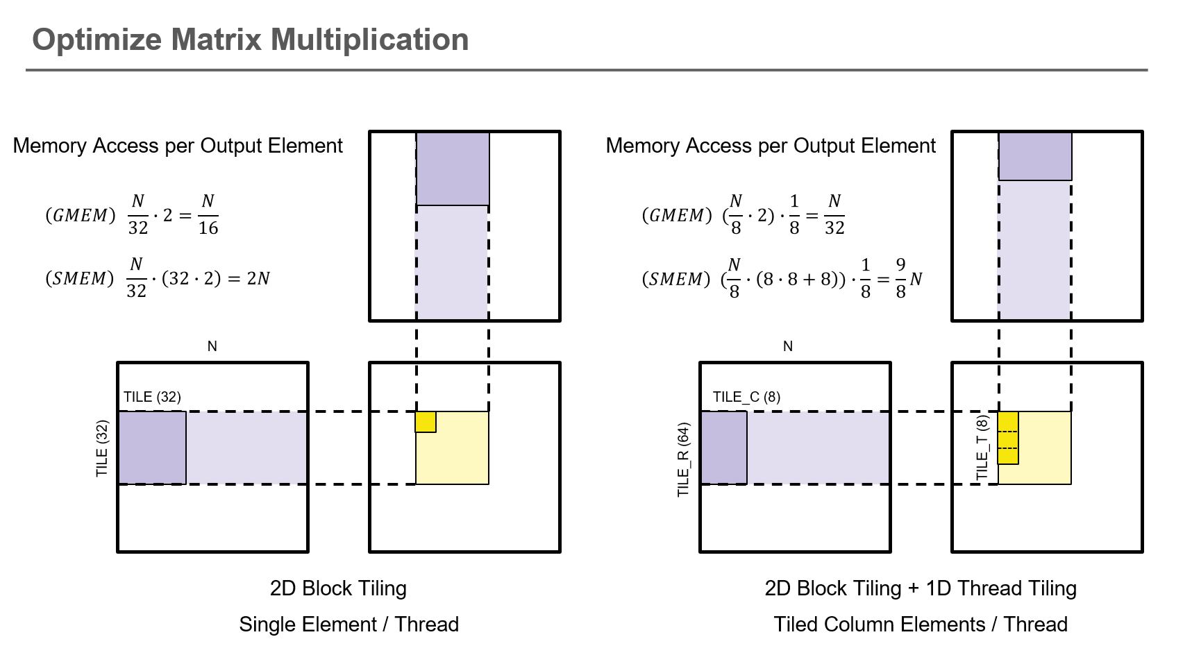
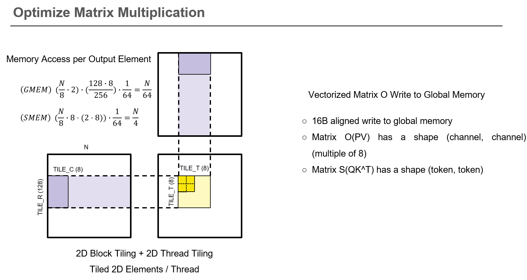
<p><img src="/images/2025-12-17/tiling.png" alt="Fig.1 Memory Tiling Optimization" />
<img src="/images/2025-12-17/tiling2.png" alt="Fig.2 Memory Tiling Optimization" /></p>

<p>A tiled matrix multiplication strategy was first implemented by loading partial matrices into shared memory, computing partial products, and accumulating the results.</p>

<p>Since the (QK^T) operation requires multiplication with a transposed (K) matrix, data were loaded from global memory in a non-transposed format to maximize memory coalescing. The transposition was then performed when storing the data into shared memory.</p>

<p>To further improve performance, 1D and 2D tiling techniques previously used in matrix multiplication were applied. These approaches reduce the frequency of accesses to both global memory and shared memory, thereby increasing data reuse and improving execution speed compared to a naïve shared-memory implementation.</p>

<p><img src="/images/2025-12-17/tiling2.png" alt="Fig.3 Vectorization" />
Furthermore, although CUDA compilers do not automatically vectorize accesses to contiguous global memory locations, vectorized memory access functions were explicitly utilized, resulting in additional performance improvements.</p>

<h2 id="12-warp-level-optimization-using-wmma">1.2 Warp-Level Optimization Using WMMA</h2>

<p>Profiling results revealed that global memory loading was the primary bottleneck for FP32 computation, whereas computation itself became the dominant bottleneck in FP16. Since most modern deep learning models operate in low-precision formats such as FP16 and BF16, optimization efforts focused on FP16 execution.</p>

<p>GPUs follow a SIMT execution model. Threads within an SM execute the same instruction stream, and instructions are scheduled at the warp level. On modern NVIDIA GPUs, a warp consists of 32 threads.</p>

<p>Leveraging this execution model, the matrix multiplication operations within scaled dot-product attention were scheduled at the warp level. Since warps can execute independently and in parallel, this approach increases the overall degree of parallelism.</p>

<p>In addition, modern GPUs contain Tensor Cores designed specifically to accelerate matrix-matrix multiplication. Tensor Cores operate at the warp level, and NVIDIA provides WMMA APIs for accessing them. These WMMA operations were integrated into the matrix multiplication stage of scaled dot-product attention.</p>

<p>As a result, on the RTX 5080 GPU, the optimized implementation achieved a runtime of 0.87 ms for a sequence length of 512, matching the performance of PyTorch. However, for longer sequence lengths such as 1024 and 2048, the implementation remained approximately 1–4 ms slower than the PyTorch baseline.</p>

<h2 id="13-instruction-level-optimization-using-ptx">1.3 Instruction-Level Optimization Using PTX</h2>
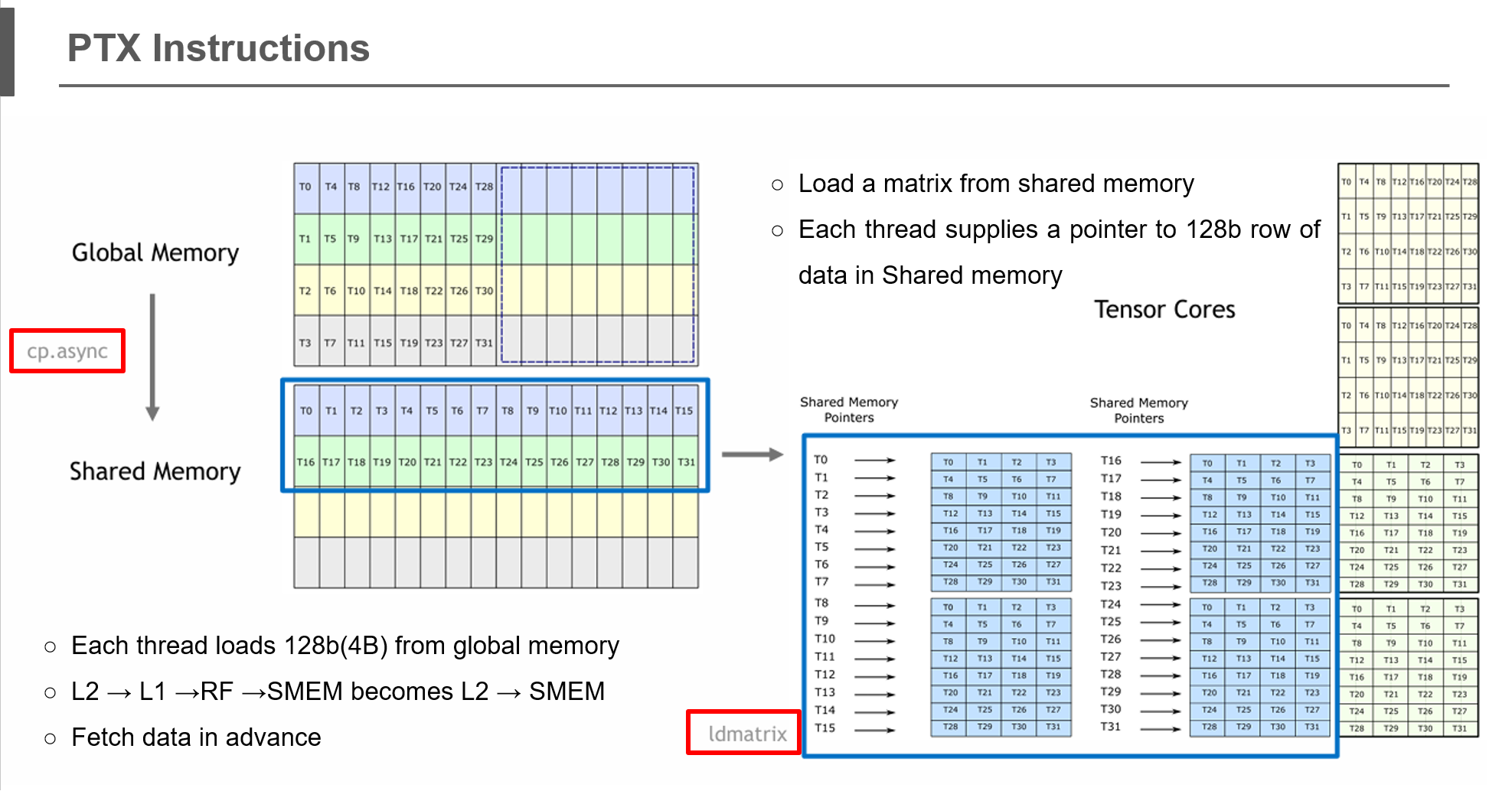
<p><img src="/images/2025-12-17/ptx.png" alt="Fig.4 PTX" /></p>

<p>Despite multiple optimization stages, the implementation remained slower than the PyTorch baseline. Further profiling revealed a significant number of shared memory bank conflicts.</p>

<p>The performance gap became increasingly pronounced as matrix dimensions increased, suggesting that bank conflicts were a major bottleneck.</p>

<p>With WMMA, thread access patterns inside a warp cannot be directly controlled, making it difficult to avoid multiple threads accessing the same shared memory bank.</p>

<p>To address this issue, PTX instructions provided by NVIDIA were employed. NVIDIA provides instructions that permute addresses when storing data into shared memory. By utilizing these instructions, threads within the same warp were forced to access different shared memory banks, effectively eliminating bank conflicts.</p>

<p>As a result, the optimized implementation outperformed the PyTorch baseline across all sequence lengths that could fit within the memory capacity of the RTX 5080 GPU, up to a sequence length of 4096.</p>

<p>In particular, for sequence length 4096, PyTorch required 50.18 ms, whereas the PTX-optimized custom kernel completed in 39.92 ms, achieving approximately a 10 ms speedup.</p>

<h2 id="14-softmax-optimization">1.4 Softmax Optimization</h2>
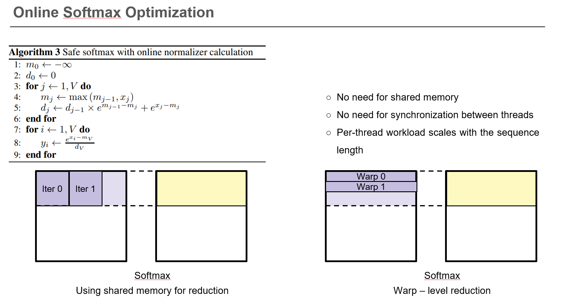
<p><img src="/images/2025-12-17/softmax.png" alt="Fig.5 Softmax Optimization" />
While optimizing matrix multiplication, kernel-level profiling indicated that the softmax operation constituted a major performance bottleneck.</p>

<p>An online softmax algorithm was initially implemented to simultaneously compute the running maximum, perform numerical stabilization, and accumulate the normalization term. However, this approach required storing intermediate values in shared memory and introduced multiple synchronization barriers through repeated <code class="language-plaintext highlighter-rouge">__syncthreads()</code> calls.</p>

<p>To eliminate these overheads, the warp-level execution model used in matrix multiplication was applied to softmax computation as well. Each warp independently processed one softmax operation, removing the need for shared memory communication and synchronization.</p>

<p>Through this design, a softmax kernel with performance comparable to PyTorch’s implementation was achieved.</p>

<h1 id="2-implementation-of-attention-linear-projection-using-cuda-kernels">2. Implementation of Attention Linear Projection Using CUDA Kernels</h1>

<p>Matrix multiplication kernels were implemented to perform the Q/K/V projections and the output linear projection in the attention mechanism.</p>

<h2 id="21-shared-memory-tiling">2.1 Shared Memory Tiling</h2>

<p>A cache-blocked tiled GEMM kernel was implemented using shared memory. Input and weight matrices were loaded into shared memory tile-by-tile, and partial products were accumulated locally.</p>

<p>The primary objective was to reduce redundant global memory accesses and improve arithmetic intensity through tile reuse.</p>

<p>During implementation, considerations such as shared memory bank conflicts and boundary handling for incomplete tiles were required.</p>

<p>Performance evaluation showed that the implementation remained slower than cuBLAS, indicating the need for further optimization. Profiling suggested that memory access overhead rather than computational workload was the dominant bottleneck, motivating the adoption of register tiling as the next optimization stage.</p>

<p>In addition, accuracy verification revealed errors significantly exceeding acceptable tolerance levels, indicating issues in the computation process that required further investigation.</p>

<h2 id="22-accuracy-issues">2.2 Accuracy Issues</h2>

<p>For correctness verification, the outputs of the custom kernel were compared against cuBLAS results using the maximum absolute difference metric.</p>

<p>It was discovered that cuBLAS assumes column-major matrix layouts by default, whereas the custom kernel interpreted matrices in row-major format. This layout mismatch effectively introduced an implicit transpose operation and resulted in substantial numerical discrepancies.</p>

<p>After aligning the matrix layouts, the accuracy issue was resolved. Boundary conditions were also carefully examined to ensure that no out-of-bound accesses or missing computations occurred near tile boundaries.</p>

<h2 id="23-register-block-tiling-1d-and-2d">2.3 Register Block Tiling: 1D and 2D</h2>

<p>Register block tiling was introduced by allowing each thread to accumulate a subset of output elements directly in registers.</p>

<p>Both 1D and 2D block tiling strategies were implemented sequentially, increasing per-thread workload and improving data reuse.</p>

<p>Compared with the shared-memory-only implementation, register tiling improved performance by approximately 40%.</p>

<p>While 2D tiling further increases data reuse relative to 1D tiling, its effectiveness depends on the underlying bottleneck. If shared memory bandwidth or bank conflicts dominate execution time, additional tiling may provide limited benefits. Furthermore, increased register usage can reduce achieved occupancy due to higher register pressure.</p>
<p>These observations highlight the importance of balancing tile dimensions, shared memory utilization, and register consumption through careful parameter tuning.</p>

<h2 id="24-vectorization">2.4 Vectorization</h2>

<p>To improve memory efficiency, vectorized memory accesses were introduced.</p>

<p>Contiguous memory locations were loaded as vectorized data structures both during global-to-shared memory transfers and shared-to-register transfers. This reduced the number of memory transactions and improved memory throughput.</p>

<p>Performance measurements showed approximately a 30% improvement after vectorization.</p>

<p>Additional optimization opportunities were identified through shared memory indexing refinements and tuning of tile parameters such as BK.</p>

<h1 id="3-implementation-of-qkv-projection-using-cuda-kernels">3. Implementation of Q/K/V Projection Using CUDA Kernels</h1>

<p>A GEMM kernel was implemented for generating Q, K, and V projections in the attention mechanism.</p>

<p>The target problem consisted of FP16 input matrices (A) and (B), FP32 accumulation matrices (C) and (D), and matrix dimensions (M = N = K = 4096). The ultimate objective was to achieve performance comparable to cuBLAS.</p>

<h2 id="31-naïve-mma-kernel">3.1 Naïve MMA Kernel</h2>

<h3 id="311-kernel-design">3.1.1 Kernel Design</h3>

<p>The simplest approach directly invokes the PTX instruction</p>

<div class="language-text highlighter-rouge"><div class="highlight"><pre class="highlight"><code>mma.sync.aligned.m16n8k16.row.col.f32.f16.f16.f32
</code></pre></div></div>

<p>to execute Tensor Core operations.</p>

<p>On Ada GPUs, each SM contains four warp schedulers and Tensor Cores, requiring at least four warps per thread block to fully utilize the hardware.</p>

<p>A thread block consisting of (16 \times 16) threads was used, yielding a total of eight warps. These warps were arranged as a (2 \times 4) grid, collectively computing a (32 \times 32) output tile.</p>

<p>Each warp computes a (16 \times 8) output tile, and all Tensor Core operations are issued through inline PTX assembly rather than CUDA high-level APIs.</p>

<h3 id="312-data-movement-and-computation">3.1.2 Data Movement and Computation</h3>

<p>The naïve kernel employs a straightforward data movement strategy.</p>

<p>Each thread independently loads FP16 elements from global memory into shared memory. These accesses are neither contiguous nor aligned, resulting in poor global memory utilization.</p>

<p>Subsequently, data are loaded from shared memory into registers. Since multiple threads within the same warp frequently access the same shared memory bank, substantial bank conflicts occur.</p>

<p>Because each loaded element participates in only a single MMA operation, data reuse is extremely limited. Consequently, memory access costs dominate execution time and Tensor Core resources remain underutilized.</p>

<h3 id="313-performance-analysis">3.1.3 Performance Analysis</h3>

<p>Kernel 1.0 achieved an execution time of 4680 µs and a throughput of 29.4 TFLOP/s.</p>

<p>This corresponds to approximately 19.1% of cuBLAS performance and 17.8% of the theoretical peak performance of the RTX 4090.</p>

<p>Nsight Compute analysis identified shared memory throttling, synchronization barriers, and long-scoreboard stalls caused by global memory loads as the primary bottlenecks.</p>

<p>On average, each MMA instruction required approximately 180 cycles, substantially higher than the theoretical minimum of 32 cycles.</p>

<h3 id="314-basic-tiling-improvement-kernel-11">3.1.4 Basic Tiling Improvement: Kernel 1.1</h3>

<p>Applying 2× tiling along both the M and N dimensions allows each warp to execute four MMA operations per iteration.</p>

<p>As a result, the output tile size expands from (32 \times 32) to (64 \times 64).</p>

<p>This simple modification reduces execution time to 2400 µs and increases throughput to 57.3 TFLOP/s, achieving approximately 37.3% of cuBLAS performance.</p>

<p>However, global memory inefficiencies and shared memory bank conflicts remain unresolved, limiting further performance gains.</p>

<h2 id="32-vectorized-loads-and-permuted-shared-memory-layout">3.2 Vectorized Loads and Permuted Shared Memory Layout</h2>

<h3 id="321-motivation">3.2.1 Motivation</h3>

<p>The primary bottlenecks of Kernel 1 were inefficient global memory accesses, shared memory bank conflicts, and low data reuse.</p>

<p>To address these issues, techniques inspired by CUTLASS were adopted, including 128-bit vectorized loads using <code class="language-plaintext highlighter-rouge">uint4</code>, permuted shared memory layouts, and warp-level loading via <code class="language-plaintext highlighter-rouge">ldmatrix</code>.</p>

<h3 id="322-vectorized-global-memory-loads">3.2.2 Vectorized Global Memory Loads</h3>

<p>Tensor Cores operate on 128-bit vector fragments. Therefore, eight consecutive FP16 values along the K dimension were packed into a single <code class="language-plaintext highlighter-rouge">uint4</code> load.</p>

<p>Matrices A and B were stored in row-major and column-major formats, respectively. Warp-level loading ensured fully coalesced global memory accesses and significantly improved bandwidth utilization.</p>

<h3 id="323-permuted-shared-memory-layout">3.2.3 Permuted Shared Memory Layout</h3>

<p>Shared memory consists of 32 banks with a width of 4 bytes.</p>

<p>Since a <code class="language-plaintext highlighter-rouge">uint4</code> occupies 16 bytes, naïve row-major storage would generate bank conflicts during warp-wide accesses.</p>

<p>To avoid this, an XOR-based permutation was applied:</p>

<div class="language-text highlighter-rouge"><div class="highlight"><pre class="highlight"><code>store_column = (laneID mod 8) XOR floor(laneID / 8)
</code></pre></div></div>

<p>This permutation eliminates bank conflicts both during global-to-shared stores and subsequent <code class="language-plaintext highlighter-rouge">ldmatrix</code> loads.</p>

<h3 id="324-register-loading-using-ldmatrix">3.2.4 Register Loading Using <code class="language-plaintext highlighter-rouge">ldmatrix</code></h3>

<p>The instruction <code class="language-plaintext highlighter-rouge">ldmatrix.sync.aligned</code> loads (8 \times 128)-bit blocks from shared memory and transforms them into Tensor Core register fragments.</p>

<p>A tiles are loaded using <code class="language-plaintext highlighter-rouge">ldmatrix.x4</code>, while B tiles are loaded using <code class="language-plaintext highlighter-rouge">ldmatrix.x2</code>.</p>

<p>Because of the permuted shared memory layout, all threads access distinct banks, eliminating loading stalls.</p>

<h3 id="325-performance-improvements">3.2.5 Performance Improvements</h3>

<p>Kernel 2.0 reduced execution time to 1080 µs and achieved 127.3 TFLOP/s, corresponding to 82.9% of cuBLAS performance.</p>

<p>Kernel 2.1 further improved register reuse by loading A tiles only once, reducing execution time to 1030 µs and increasing throughput to 133.4 TFLOP/s, or 86.9% of cuBLAS performance.</p>

<p>Average MMA latency decreased to 38 cycles, and the dominant bottleneck shifted from memory stalls to Tensor Core pipeline utilization.</p>

<h2 id="33-n-stage-global-to-shared-pipeline">3.3 N-Stage Global-to-Shared Pipeline</h2>

<h3 id="331-motivation">3.3.1 Motivation</h3>

<p>Although Kernel 2 significantly improved performance, long-scoreboard stalls caused by global memory loads remained.</p>

<p>To further hide memory latency, an N-stage global-to-shared pipeline based on <code class="language-plaintext highlighter-rouge">cp.async</code> was introduced.</p>

<h3 id="332-cpasync-pipeline-design">3.3.2 <code class="language-plaintext highlighter-rouge">cp.async</code> Pipeline Design</h3>

<p>The <code class="language-plaintext highlighter-rouge">cp.async</code> instruction enables asynchronous data transfers from global memory to shared memory.</p>

<p>A circular buffer consisting of <code class="language-plaintext highlighter-rouge">N_STAGES</code> shared-memory buffers was allocated, and synchronization was controlled through <code class="language-plaintext highlighter-rouge">cp.async.commit_group</code> and <code class="language-plaintext highlighter-rouge">cp.async.wait_group</code>.</p>

<p>During execution, MMA operations on the current stage overlap with global-to-shared prefetching for the next stage, effectively hiding memory latency.</p>

<h3 id="333-performance-results-and-extended-tiling">3.3.3 Performance Results and Extended Tiling</h3>

<p>Kernel 3.0 achieved an execution time of 1000 µs and a throughput of 137.4 TFLOP/s, corresponding to 89.5% of cuBLAS performance.</p>

<p>Kernel 3.1 further expanded tiling along both M and N dimensions by 4×, increasing MMA density per warp.</p>

<p>As a result, execution time decreased to 895 µs, matching the performance of cuBLAS.</p>

<p>Warp-state analysis showed that most stalls were due to Tensor Core pipeline limitations, and average MMA latency reached 34.2 cycles, approaching the theoretical minimum of 32 cycles.</p>

<h3 id="334-summary">3.3.4 Summary</h3>

<p>By combining an N-stage global-to-shared pipeline with large-scale tiling, global memory latency was effectively hidden and Tensor Core utilization was maximized.</p>

<p>These results demonstrate that achieving near-theoretical Tensor Core performance requires careful memory-layout design, warp-level data movement optimization, and asynchronous pipeline scheduling.</p>

<h1 id="references">References</h1>
<p>[1] <a href="https://www.spatters.ca/mma-matmul">https://www.spatters.ca/mma-matmul</a></p>

<p>[2] <a href="https://siboehm.com/articles/22/CUDA-MMM">https://siboehm.com/articles/22/CUDA-MMM</a></p>]]></content><author><name>Seoyoon Chae</name><email>sychaeee@g.skku.edu</email></author><summary type="html"><![CDATA[Implemented and optimized CUDA kernels for scaled dot-product attention, attention linear projection, and Q/K/V projection.]]></summary></entry><entry><title type="html">[ISOCC 2025] LLM on FPGA: Squeezing Language Models by Quantization and Multi-Query Attention and Its Efficient Hardware Architecture</title><link href="https://chae-sy.github.io/LLM-on-FPGA/" rel="alternate" type="text/html" title="[ISOCC 2025] LLM on FPGA: Squeezing Language Models by Quantization and Multi-Query Attention and Its Efficient Hardware Architecture" /><published>2025-10-16T00:00:00+00:00</published><updated>2025-10-16T00:00:00+00:00</updated><id>https://chae-sy.github.io/LLM-on-FPGA</id><content type="html" xml:base="https://chae-sy.github.io/LLM-on-FPGA/"><![CDATA[<p>Delighted to share that my research has been accepted to an oral session of ISOCC 2025 – 22th International SoC Design Conference! (presented on October 16, 2025)</p>

<p>you can find the whole paper : LLM on FPGA: Squeezing Language Models by Quantization and Multi-Query Attention and its Efficient Hardware Architecture <a href="https://ieeexplore.ieee.org/abstract/document/11329964">link</a></p>

<p>The paper got recognized “For enabling analytical evaluation of various quantization schemes (SmoothQuant and QLoRA) and implementing on-chip caches of large language models without siginificant accuracy drop by using Multi-Query Attention and efficient RTL design.”</p>

<h2 id="llm-on-fpga-squeezing-language-models-by-quantization-and-multi-query-attention-and-its-efficient-hardware-architecture">LLM on FPGA: Squeezing Language Models by Quantization and Multi-Query Attention and Its Efficient Hardware Architecture</h2>

<p><strong>Authors:</strong></p>

<p>Seoyoon Chae (Dept. of Electronic and Electrical Engineering, Sungkyunkwan University)</p>

<p>Taewook Kang (Dept. of Semiconductor Convergence Engineering, Sungkyunkwan University)</p>

<p>🔗 <strong>Code:</strong> <a href="https://github.com/chae-sy/squeezing_lm">https://github.com/chae-sy/squeezing_lm</a></p>

<hr />

<h2 id="abstract">Abstract</h2>

<p>We present an <strong>on-chip implementation</strong> of a compressed Transformer-based language model on a <strong>Xilinx Artix-7 FPGA</strong>.</p>

<p>Our main contributions are:</p>

<ol>
  <li><strong>Hybrid compression:</strong> Combining <strong>4-bit quantization</strong> and <strong>multi-query attention (MQA)</strong> compresses the KV cache by <strong>8×</strong>, supporting sequences up to <strong>256 tokens</strong>.</li>
  <li><strong>Streaming hardware design:</strong> A <strong>Verilog implementation</strong> of pre-layernorm, attention, and feed-forward sublayers optimized with <strong>BRAM</strong> and <strong>DSP utilization</strong>.</li>
  <li><strong>Post-synthesis performance:</strong> Achieving <strong>4.4 K tokens/s</strong> at 250 MHz with <strong>31.9% BRAM</strong> and <strong>85% DSP</strong> utilization.</li>
</ol>

<p>This prototype enables <strong>fully on-chip generative inference</strong>, advancing privacy-preserving and edge-deployable large language models.</p>

<p><strong>Keywords:</strong> Large Language Model (LLM), Quantization, Multi-Query Attention, Transformer Accelerator, FPGA, On-Device Inference, Hardware–Software Co-Design</p>

<hr />

<h2 id="1-introduction">1. Introduction</h2>

<p>Transformer-based <strong>large language models (LLMs)</strong> achieve state-of-the-art performance but require substantial compute and memory resources
Autoregressive generation typically caches <strong>key–value (KV) tensors</strong>, reducing attention complexity from <em>O(S²d)</em> to <em>O(Sd)</em> per token. However, storing 8-bit KV tensors on-chip severely limits sequence length.</p>

<p>For example, with <strong>608 KiB BRAM</strong> on an <strong>Artix-7 FPGA</strong>, the on-chip KV capacity is:</p>

\[\text{Token capacity}=\frac{608\,\text{KiB}}{12\,\text{layers} \times 2\,\text{KV tensors} \times 768\,\text{B}}\approx 33\,\text{tokens.}\]

<p>To overcome this limitation, we integrate <strong>sub-8-bit quantization</strong> and <strong>MQA</strong> to compress the KV cache over <strong>8×</strong>, enabling <strong>256-token inference</strong> without DRAM.</p>

<p><strong>Key contributions:</strong></p>

<ul>
  <li><strong>4-bit KV quantization</strong> using SmoothQuant + LoRA-QAT achieves near-lossless accuracy (&lt; 0.02 drop).</li>
  <li><strong>MQA (shared K/V across heads)</strong> cuts bandwidth while preserving quality.</li>
  <li><strong>FPGA co-design:</strong> A streaming Transformer block implemented entirely in Verilog.</li>
</ul>

<hr />

<h2 id="2-related-work">2. Related Work</h2>

<p>Previous research explored:</p>

<ul>
  <li>Multi-head attention acceleration on systolic arrays [2].</li>
  <li>ASICs using per-vector 4-bit scaling [3].</li>
  <li>FPGA frameworks applying pruning [4].</li>
</ul>

<p>However, none jointly exploit <strong>sub-8-bit quantization</strong> and <strong>KV caching</strong> for <strong>generative LLM inference</strong> under FPGA-scale memory constraints.</p>

<hr />

<h2 id="3-model-compression-methodology">3. Model Compression Methodology</h2>

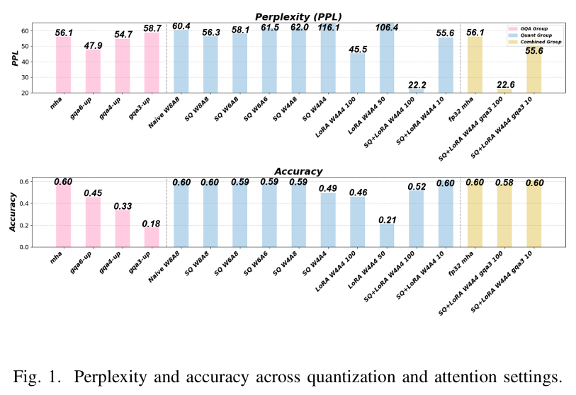
<p><img src="/images/2025-10-16/image.png" alt="image.png" /></p>

<h3 id="31-smoothquant-for-range-equalization">3.1 SmoothQuant for Range Equalization</h3>

<p>SmoothQuant [5] was used to mitigate activation outliers before quantization.</p>

<ul>
  <li>Stable results for <strong>W8A8–W6A6</strong> (PPL ≈ 60, Accuracy ≈ 0.6).</li>
  <li>Instability observed at <strong>W4A4</strong> (PPL = 116.1, Accuracy = 0.49).</li>
</ul>

<h3 id="32-lora-based-quantization-aware-training">3.2 LoRA-Based Quantization-Aware Training</h3>

<p>LoRA adapters (rank = 8) were inserted into Q/K/V projections and fine-tuned on <strong>WikiText-2</strong> for 10–100 steps (frozen backbone).</p>

<ul>
  <li>PPL = 45.5 after 100 steps.</li>
  <li>Combining with SmoothQuant reduced PPL to <strong>22.2</strong> (100 steps) and <strong>55.6</strong> (10 steps).</li>
</ul>

<h3 id="33-multi-query-attention-mqa">3.3 Multi-Query Attention (MQA)</h3>

<p>Standard <strong>MHA</strong> computes separate K/V per head → high memory cost.</p>

<p><strong>MQA</strong> shares K/V across all heads; <strong>GQA</strong> shares within groups.</p>

<p>In our experiments:</p>

<ul>
  <li><strong>Group-3 MQA</strong> saved significant memory.</li>
  <li>Slight trade-off: +2.6 PPL vs. baseline MHA.</li>
</ul>

<p><strong>Result Summary:</strong></p>

<table>
  <thead>
    <tr>
      <th>Configuration</th>
      <th>Training Steps</th>
      <th>PPL</th>
      <th>Accuracy</th>
    </tr>
  </thead>
  <tbody>
    <tr>
      <td>W4A4 + SmoothQuant (10 steps) + G3 MQA</td>
      <td>10</td>
      <td>55.6</td>
      <td>0.60</td>
    </tr>
    <tr>
      <td>W4A4 + SmoothQuant (100 steps) + G3 MQA</td>
      <td>100</td>
      <td><strong>22.6</strong></td>
      <td>0.58</td>
    </tr>
  </tbody>
</table>

<hr />

<h2 id="4-hardware-architecture">4. Hardware Architecture</h2>

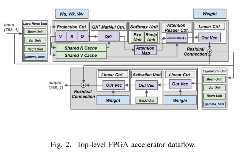
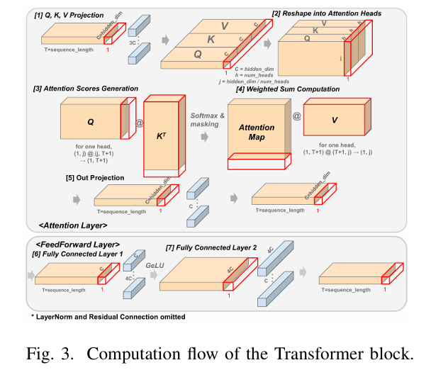
<p>The hardware pipeline consists of <strong>pre-layernorm</strong>, <strong>attention</strong>, and <strong>feed-forward network (FFN)</strong> units</p>

<p><img src="/images/2025-10-16/image%201.png" alt="image.png" /></p>

<p><img src="/images/2025-10-16/image%202.png" alt="image.png" /></p>

<h3 id="41-pre-layernorm">4.1 Pre-LayerNorm</h3>

<p>Computes per-channel mean/variance, approximates \(\frac{1}{\sqrt{\sigma^2 + \epsilon}}\) using a <strong>LUT-based reciprocal square root</strong>, and applies <strong>4-bit affine parameters</strong> (γ, β).</p>

<h3 id="42-attention-and-ffn-engines">4.2 Attention and FFN Engines</h3>

<ul>
  <li><strong>Attention Unit:</strong>
    <ul>
      <li>Generates concatenated Q/K/V via 1×1 convolution.</li>
      <li>Stores 4-bit compressed K/V in shared BRAM.</li>
      <li>Computes Q–K dot-products on a <strong>PE array</strong>.</li>
      <li>Applies masked softmax using <strong>exp/reciprocal LUTs</strong>.</li>
      <li>Produces context vector via weighted sum over V.</li>
    </ul>
  </li>
  <li><strong>Feed-Forward Network (FFN):</strong>
    <ul>
      <li>Expands C → 4C → C.</li>
      <li>Uses LUT-based GELU activation.</li>
      <li>Implemented as <strong>streaming matrix-vector (mat-vec) computations</strong> using DSPs and BRAM.</li>
    </ul>
  </li>
</ul>

<h3 id="43-resource-utilization">4.3 Resource Utilization</h3>

<table>
  <thead>
    <tr>
      <th>Resource</th>
      <th>Used</th>
      <th>Available</th>
      <th>Utilization (%)</th>
    </tr>
  </thead>
  <tbody>
    <tr>
      <td><strong>DSP slices</strong></td>
      <td>204</td>
      <td>240</td>
      <td><strong>85.0</strong></td>
    </tr>
    <tr>
      <td><strong>BRAM</strong></td>
      <td>193.5 KB</td>
      <td>608 KB</td>
      <td><strong>31.9</strong></td>
    </tr>
    <tr>
      <td><strong>LUTs</strong></td>
      <td>10,000</td>
      <td>63,400</td>
      <td><strong>15.7</strong></td>
    </tr>
  </tbody>
</table>

<hr />

<h2 id="5-evaluation">5. Evaluation</h2>

<ul>
  <li><strong>Platform:</strong> Xilinx Artix-7 100T (CSG324)</li>
  <li><strong>Tool:</strong> Vivado 2018.3</li>
  <li><strong>Clock Frequency:</strong> 250 MHz</li>
</ul>

<p>The fully pipelined design sustains <strong>1 token per cycle</strong> (after pipeline fill), reaching <strong>4.4 K tokens/s</strong> throughput.</p>

<p>On-chip memory supports <strong>sequence length ≤ 256 tokens</strong>, entirely without external DRAM.</p>

<hr />

<h2 id="6-conclusion-and-future-work">6. Conclusion and Future Work</h2>

<p>This work demonstrates the <strong>first fully on-chip FPGA-based LLM inference</strong> using:</p>

<ul>
  <li><strong>4-bit quantization</strong>,</li>
  <li><strong>Multi-Query Attention</strong>, and</li>
  <li>A <strong>streaming Verilog architecture</strong>.</li>
</ul>

<p>The prototype achieves <strong>real-time generation</strong> within <strong>31.9% BRAM</strong> and <strong>85% DSP</strong> budgets.</p>

<p>Future directions include:</p>

<ul>
  <li>Scaling to larger LLMs,</li>
  <li><strong>Mixed-precision inference</strong>, and</li>
  <li><strong>Energy-efficiency optimization</strong>.</li>
</ul>

<hr />

<h2 id="references">References</h2>

<ol>
  <li>Vaswani et al., <em>“Attention Is All You Need,”</em> NeurIPS 2017.</li>
  <li>Lu et al., <em>“Hardware Accelerator for Multi-Head Attention and FFN,”</em> IEEE SOCC 2020.</li>
  <li>Keller et al., <em>“A 95.6-TOPS/W Inference Accelerator with 4-bit Quantization in 5 nm,”</em> IEEE JSSC 2023.</li>
  <li>Zhang et al., <em>“Algorithm-Hardware Co-Design of Attention on FPGA Devices,”</em> ACM TECS 2021.</li>
  <li>Xiao et al., <em>“SmoothQuant: Accurate and Efficient Post-Training Quantization for LLMs,”</em> ICML 2023.</li>
  <li>Hu et al., <em>“LoRA: Low-Rank Adaptation of LLMs,”</em> ICLR 2022.</li>
  <li>Shazeer, <em>“Fast Transformer Decoding: One Write-Head Is All You Need,”</em> arXiv 2019.</li>
  <li>Ainslie et al., <em>“GQA: Generalized Multi-Query Transformers,”</em> arXiv 2023.</li>
</ol>]]></content><author><name>Seoyoon Chae</name><email>sychaeee@g.skku.edu</email></author><summary type="html"><![CDATA[Delighted to share that my research has been accepted to an oral session of ISOCC 2025 – 22th International SoC Design Conference! (presented on October 16, 2025)]]></summary></entry><entry><title type="html">[tape-out project] quantized BC-ResNet models for keyword spotting and speaker verification</title><link href="https://chae-sy.github.io/Quantized-BC-ResNet-Tape-Out/" rel="alternate" type="text/html" title="[tape-out project] quantized BC-ResNet models for keyword spotting and speaker verification" /><published>2025-07-10T00:00:00+00:00</published><updated>2025-07-10T00:00:00+00:00</updated><id>https://chae-sy.github.io/Quantized-BC-ResNet-Tape-Out</id><content type="html" xml:base="https://chae-sy.github.io/Quantized-BC-ResNet-Tape-Out/"><![CDATA[<p>This post details the design and implementation of a quantized BC-ResNet-based neural network accelerator for keyword spotting (KWS) and speaker verification (SV), culminating in a successful ASIC tape-out using Samsung’s 28 nm LPP process. The project demonstrates a hardware–software co-design approach, achieving low power consumption and high accuracy for edge audio intelligence applications.</p>

<h3 id="1-introduction">1. Introduction</h3>

<p>The demand for <strong>AI processors</strong> has been rapidly increasing as machine learning applications continue to expand into edge and IoT devices. Among them, <strong>keyword spotting (KWS)</strong> and <strong>speaker verification (SV)</strong> systems have become fundamental components in modern <strong>voice-based human–machine interfaces</strong>, such as smart speakers, mobile assistants, and wearable devices. These systems enable always-on, low-power auditory perception, allowing devices to respond to wake words or authenticate users through voice features without relying on cloud processing.</p>

<p>In this research project, we aim to <strong>tape out</strong> a low-power AI processor, exploiting the synergy between neural model compression and hardware optimization for embedded audio intelligence.</p>

<hr />

<h3 id="2-related-work">2. Related Work</h3>

<p>Tan <em>et al.</em> (JSSC 2025) [1] present a <strong>1.8% FAR, 2 ms</strong> decision-latency <strong>SV-assisted KWS chip</strong> in 28 nm CMOS. They propose a <em>transfer-computing</em> model that shares convolutional layers between KWS and SV, cutting MACs and parameters by ≈1.8×. A <em>hybrid-IF-domain</em> circuit processes analog and digital features to eliminate ADC overhead, and a <em>scalable 5T-SRAM</em> reduces read/leakage power by &gt;10×. The chip achieves <strong>91.8 % accuracy</strong>, <strong>1.73 nJ/decision</strong>, and <strong>1.73 µW</strong> active power, which is the lowest among prior KWS ASICs</p>

<p>Xiao <em>et al.</em> (ISSCC 2024) [2] introduce <strong>KASP</strong>, a 55 nm <strong>KWS + SV processor</strong> using <em>adaptive beamforming</em>, <em>direction-of-arrival estimation</em>, and <em>progressive wake-up</em> to suppress human-voice noise. Its <em>Lite-FDBF</em> and <em>Lite-X-Vector</em> SV enable multi-user verification without speaker-specific training, reducing MACs by 99.7 % with only 1.4 % accuracy loss. KASP achieves <strong>96.8 % KWS accuracy</strong> and <strong>1.68 µJ/classification</strong>, representing a major advance in noise-robust, ultra-low-energy speech interfaces.</p>

<p>Unlike prior works, our work introduces a fully digitized computation and model architecture that enhances accuracy while leveraging <strong>early-exiting branches</strong> to reduce the switching activity of power-hungry digital cells, thereby achieving lower overall power consumption.</p>

<hr />

<h3 id="3-system-overview">3. System Overview</h3>

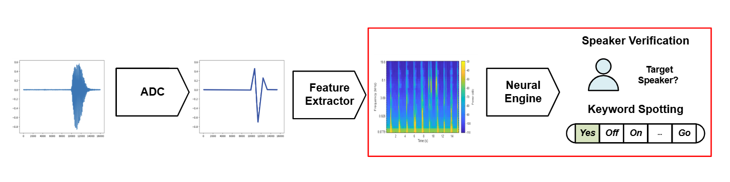
<p><img src="/images/2025-07-10/image.png" alt="Fig. 1 : Overall System Pipeline" /></p>

<p>Fig. 1 : Overall System Pipeline</p>

<p>The overall system pipeline, as illustrated in <strong>Fig. 1</strong>, consists of three main components: an <strong>Analog-to-Digital Converter (ADC)</strong>, a <strong>Feature Extractor</strong>, and a <strong>Neural Engine</strong>.</p>

<p>First, the incoming <strong>acoustic waveform</strong> is captured and digitized through the ADC, which converts the continuous analog speech signal into quantized digital samples suitable for further digital processing. These quantized signals are then passed to the <strong>Feature Extractor</strong>, which computes time–frequency representations such as <strong>Mel-spectrograms</strong> to capture the spectral characteristics of the speech signal.</p>

<p>The extracted features are subsequently fed into the <strong>Neural Engine</strong>, which performs two parallel inference tasks: <strong>Keyword Spotting (KWS)</strong> and <strong>Speaker Verification (SV)</strong>. The neural network identifies whether the spoken utterance corresponds to a predefined keyword and simultaneously verifies whether the detected voice matches a registered target speaker.</p>

<p>In this project, the <strong>Neural Engine (</strong>highlighted in the red box of Fig. 1) was fully implemented, including model quantization, digital inference pipeline, and hardware mapping. The <strong>ADC</strong> and <strong>Feature Extractor</strong> modules were developed by collaborating teams and interfaced with the neural engine for end-to-end system evaluation.</p>

<hr />

<h3 id="4-model-design">4. Model Design</h3>

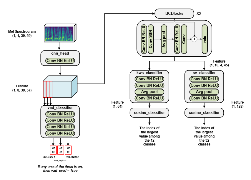
<p><img src="/images/2025-07-10/image_1.png" alt="Fig. 2 : Model Design " /></p>

<p>Fig. 2 : Model Design</p>

<p>The proposed model architecture is based on <strong>BC-ResNet</strong>, which is known for its parameter efficiency and suitability for embedded speech applications. The original BC-ResNet consists of three main components: a <strong>CNN head</strong>, a sequence of <strong>BCBlocks</strong>, and a <strong>Classifier</strong>. To jointly handle <strong>Voice Activity Detection (VAD)</strong>, <strong>Keyword Spotting (KWS)</strong>, and <strong>Speaker Verification (SV)</strong> within a unified framework, the architecture was modified as shown in <strong>Fig. 2</strong>.</p>

<p>The input <strong>Mel-spectrogram</strong> (dimension: 1 × 1 × 39 × 59) is first processed by the <strong>CNN head</strong>, which performs initial feature extraction using convolution, batch normalization, and ReLU activation. From this output, the first three time steps of the feature map are directed to the <strong>VAD classifier</strong>, composed of four sequential convolutional blocks (Conv–BN–ReLU). If any of the three VAD logits indicate activity (i.e., <code class="language-plaintext highlighter-rouge">vad_pred=True</code>), the subsequent processing stages are activated.</p>

<p>In the next stage, the complete feature map is passed through three stacked <strong>BCBlocks</strong>, each consisting of a <strong>Conv–BN–ReLU</strong>, <strong>Conv–SSN (Sub-Spectral Normalization)</strong>, <strong>Average Pooling</strong>, and an additional <strong>Conv–BN–ReLU</strong> sequence, with skip connections to preserve feature continuity and mitigate gradient degradation. These BCBlocks extract compact, discriminative embeddings suitable for both KWS and SV.</p>

<p>The resulting features are branched into two task-specific heads: the <strong>KWS classifier</strong> and the <strong>SV classifier</strong>. Each classifier comprises a shallow Conv–BN–ReLU stack followed by an average pooling layer, producing embedding vectors of size <strong>(1, 64)</strong> for KWS and <strong>(1, 128)</strong> for SV, respectively. These embeddings are then passed to <strong>cosine classifiers</strong>, which compute similarity scores between the embeddings and class prototypes. The index of the maximum cosine similarity determines the predicted keyword or speaker identity. For the ASIC implementation, only the neural encoder portion up to the embedding vector output was realized, while the cosine classifier was executed in software.</p>

<hr />

<h3 id="quantization-setup">Quantization Setup</h3>

<p>Quantization-aware training (QAT) was applied to reduce model precision while maintaining accuracy. Both <strong>weights and activations were quantized to 8 bits (W8A8)</strong>, with 32-bit accumulations for residual connections. Each <strong>Conv–BN–ReLU</strong> and <strong>Conv–SSN</strong> pair was fused into a single quantized operation to minimize computational overhead. All layers, including <strong>AdaptiveAvgPool2d</strong>, <strong>Fully Connected</strong>, <strong>Convolution</strong>, and <strong>Residual paths</strong>, were quantized to ensure full-integer arithmetic compatibility for hardware deployment. Per-channel scaling was applied to improve numerical stability during training and inference.</p>

<hr />

<h3 id="training-environment">Training Environment</h3>

<p>The model was trained on the <strong>Google Speech Commands v2 (GSCD)</strong> dataset using the <strong>SGD optimizer</strong> with a momentum of 0.9 and a weight decay of 1 × 10⁻³. The total number of epochs was <strong>300</strong>, including a <strong>10-epoch warmup</strong> phase. The initial learning rate was set to <strong>1.2 × 10⁻²</strong> and decayed to a lower limit of <strong>2 × 10⁻⁵</strong> following a cosine schedule.</p>

<p>Loss functions were defined using <strong>AAM-Softmax</strong>, with task-specific weighting parameters:</p>

<ul>
  <li><strong>SV loss</strong> (\(\lambda_{sv} = 0.3\))</li>
  <li><strong>KWS loss</strong> (\(\lambda_{kws} = 0.25\))</li>
  <li><strong>VAD loss</strong> (\(\lambda_{vad} = 1.0\))</li>
</ul>

<p>Formally, the total training objective was expressed as:</p>

\[\mathcal{L}_{total}
=
\lambda_{vad}\mathcal{L}_{vad}
+
\lambda_{kws}\mathcal{L}_{kws}
+
\lambda_{sv}\mathcal{L}_{sv}\]

<p>where \(\mathcal{L}_{kws}\) and \(\mathcal{L}_{sv}\) were computed using \(\operatorname{AAMSoftmaxLoss}(\text{num_classes}, \text{num_emb_dim})\) for 64- and 256-dimensional embeddings, respectively.</p>

<hr />

<h3 id="5-hardware-design">5. Hardware Design</h3>

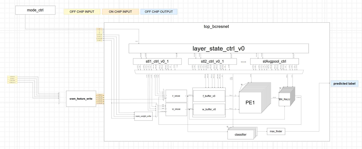
<p><img src="/images/2025-07-10/image_2.png" alt="Fig. 3 : Hardware Architecture" /></p>

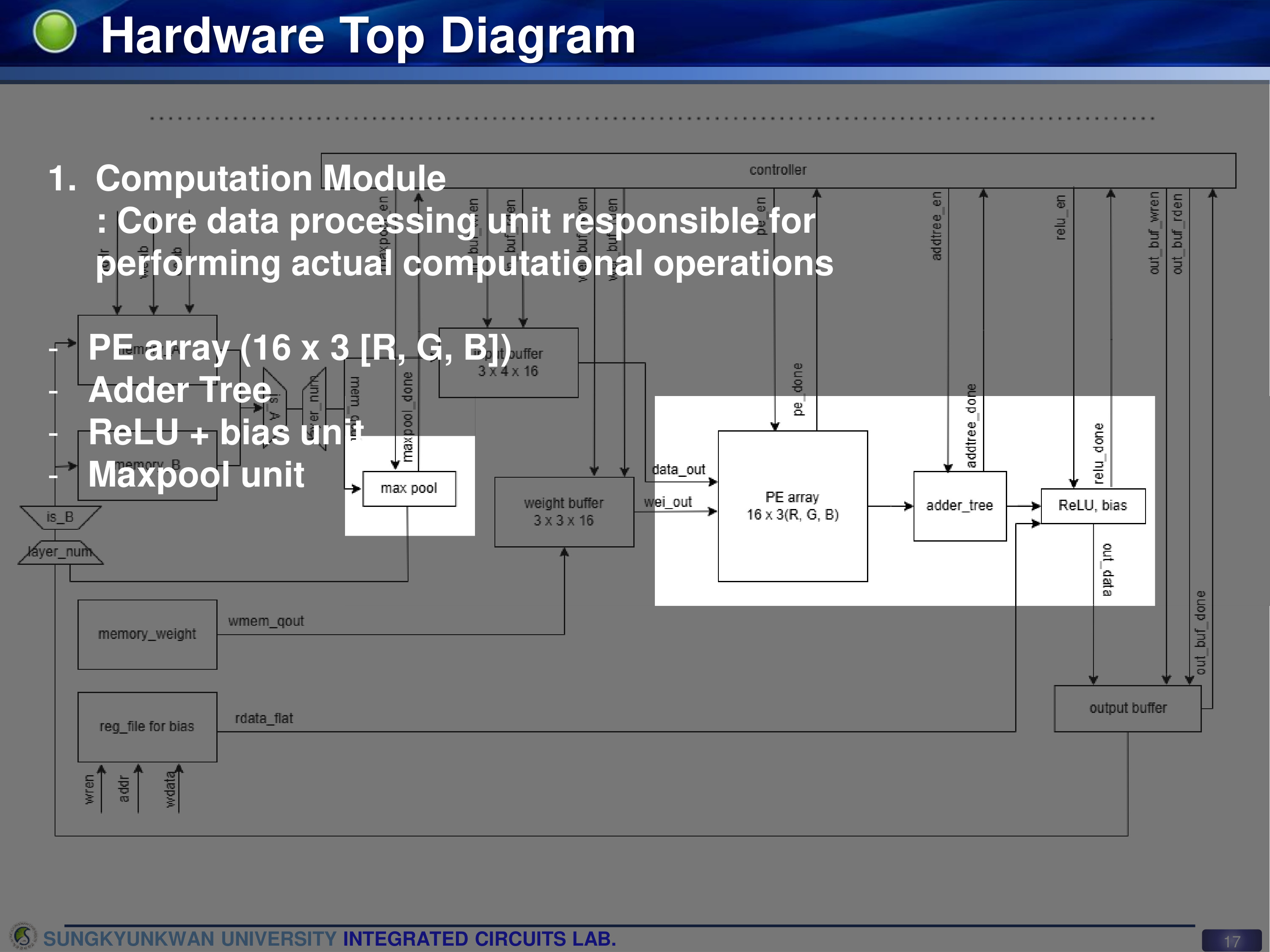
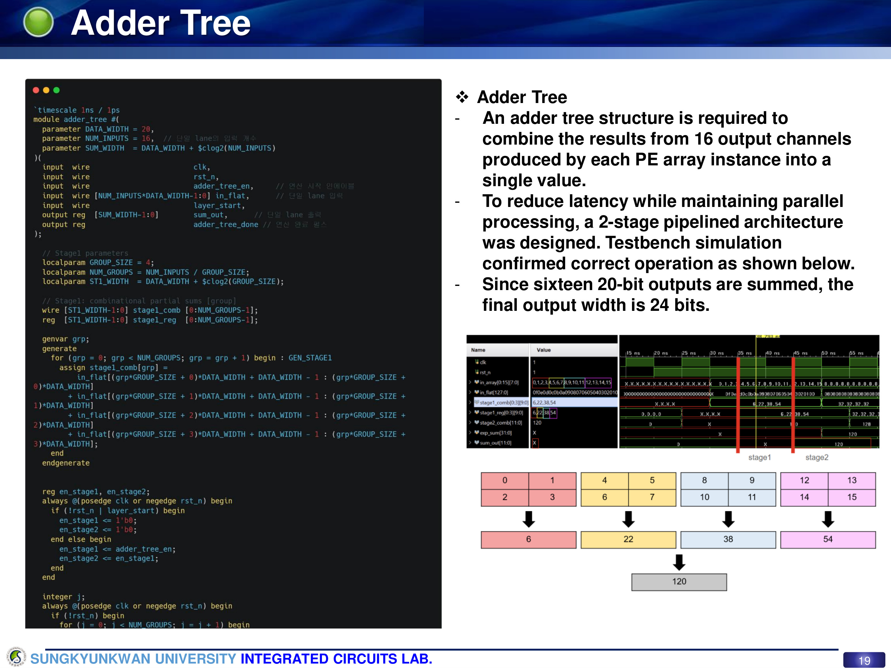
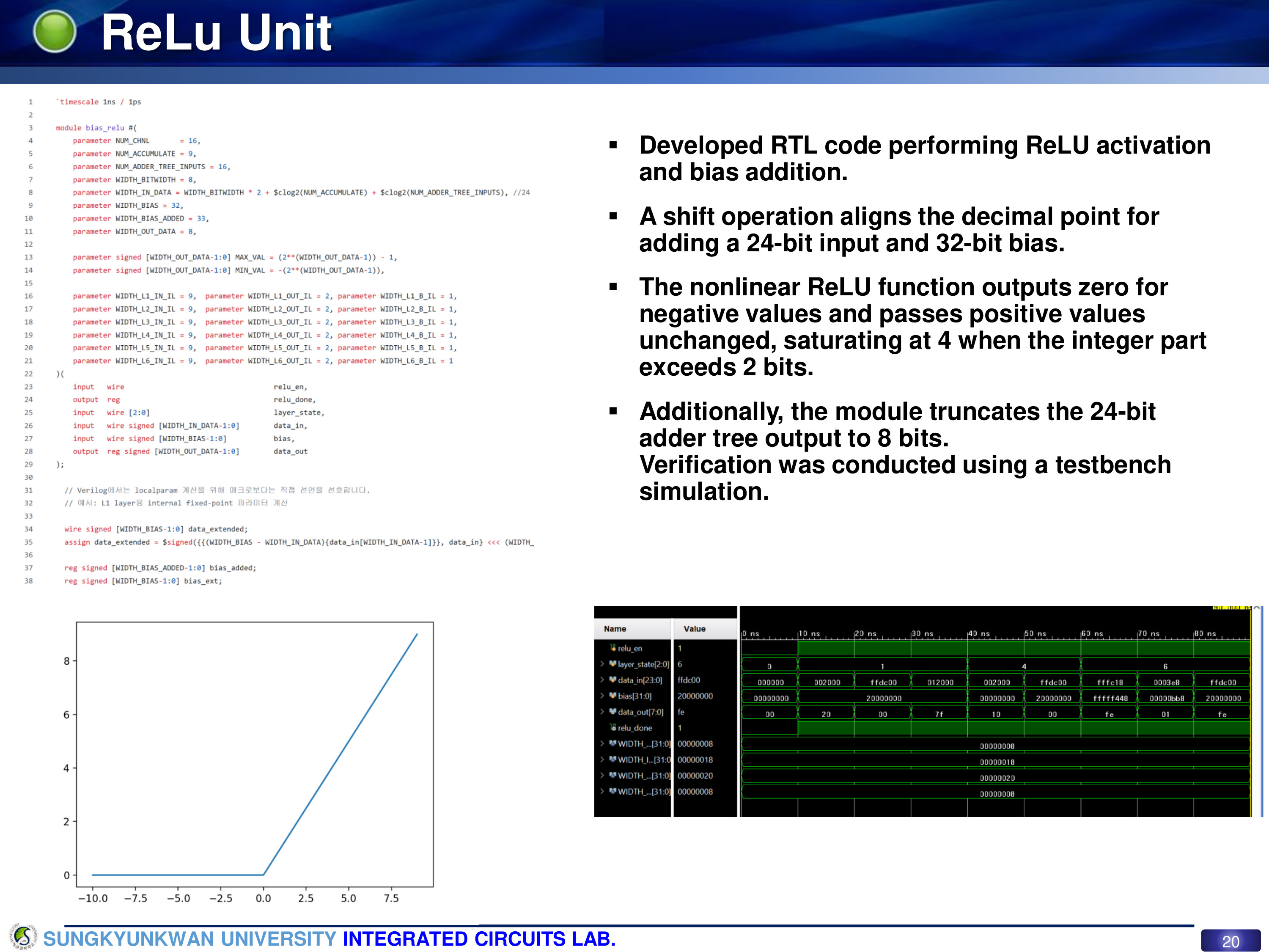
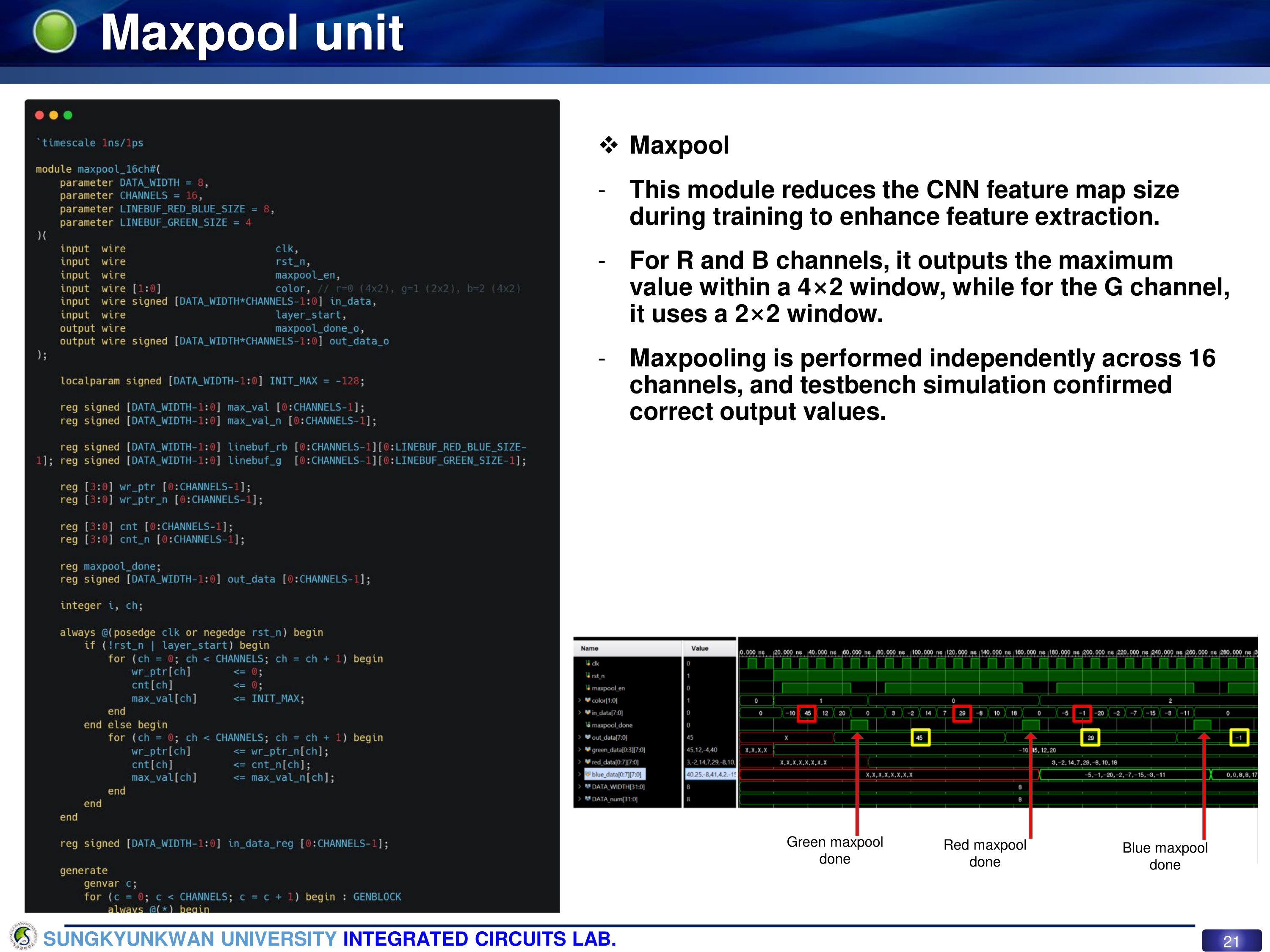
<p>Fig. 3 : Hardware Architecture</p>

<p>The proposed hardware architecture, illustrated in <strong>Fig. 3</strong>, implements the quantized BC-ResNet model for real-time keyword spotting (KWS), speaker verification (SV), and voice activity detection (VAD). The design follows a <strong>hardware–software co-design methodology</strong>, where the quantized model described in Section 4 is mapped to a custom fixed-point inference accelerator optimized for low-power edge operation.</p>

<hr />

<h3 id="51-architecture-overview">5.1 Architecture Overview</h3>

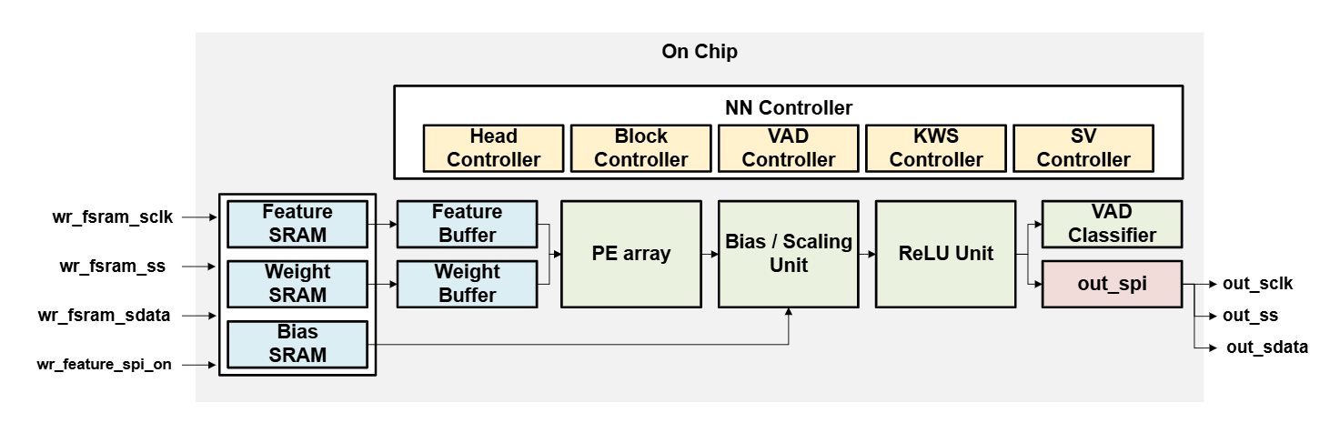
<p>The entire system is implemented <strong>on-chip</strong>, consisting of a <strong>Neural Network (NN) Controller</strong>, multiple <strong>on-chip SRAM modules</strong>, a <strong>Processing Element (PE) array</strong>, and dedicated functional units. The NN Controller is hierarchically organized into submodules: <strong>Head Controller</strong>, <strong>Block Controller</strong>, <strong>VAD Controller</strong>, <strong>KWS Controller</strong>, and <strong>SV Controller</strong>, each responsible for orchestrating the corresponding layer group in the neural network.</p>

<p>The <strong>Feature, Weight, and Bias SRAMs</strong> store the quantized feature maps, model parameters, and biases, respectively. Each SRAM is connected to a corresponding <strong>buffer</strong> to decouple memory access from computation and enable parallel data streaming. The PE array performs core multiply–accumulate (MAC) operations, and its output passes through a <strong>Bias/Scaling Unit</strong> and a <strong>ReLU Unit</strong> before being written back to SRAM or sent to the classifier. The <strong>VAD Classifier</strong> produces the final decision, which is transmitted via an SPI interface (<code class="language-plaintext highlighter-rouge">out_sclk</code>, <code class="language-plaintext highlighter-rouge">out_ss</code>, <code class="language-plaintext highlighter-rouge">out_sdata</code>).</p>

<hr />

<h3 id="52-dataflow-strategy">5.2 Dataflow Strategy</h3>

<p>The accelerator employs a <strong>channel-wise (output-stationary) dataflow</strong>, where each PE is assigned to one output channel. A total of <strong>16 PEs</strong> operate in parallel, each accumulating partial sums locally to minimize memory access overhead. The weight and feature buffers are double-buffered to enable concurrent data loading and computation, ensuring high utilization of the PE array.</p>

<p>This approach strikes a balance between compute efficiency and memory bandwidth, as weights remain stationary within the PEs while features are streamed from the Feature Buffer during each convolutional cycle.</p>

<hr />

<h3 id="53-fixed-point-arithmetic-implementation">5.3 Fixed-Point Arithmetic Implementation</h3>

<p>All arithmetic operations are performed in <strong>fixed-point precision</strong> to reduce area and power consumption.</p>

<ul>
  <li><strong>Input to PE:</strong> 8-bit feature and 8-bit weight operands</li>
  <li>
    <p><strong>Output of PE:</strong> 21-bit accumulation result</p>

    <p>The accumulated value is then processed by the <strong>Bias/Scaling Unit</strong>, which applies per-channel scaling and bias correction to restore dynamic range. The scaled result passes through the <strong>ReLU Unit</strong>, where rounding and saturation are applied. Since <strong>ReLU6 activation</strong> is adopted, the output is saturated at a maximum value of 6, preventing numerical overflow while preserving nonlinear activation effects.</p>
  </li>
</ul>

<hr />

<h3 id="54-memory-design">5.4 Memory Design</h3>

<p>The on-chip memory subsystem consists of three dedicated SRAM blocks:</p>

<ul>
  <li><strong>Feature SRAM (64 KB)</strong> – stores intermediate activation maps</li>
  <li><strong>Weight SRAM (128 KB)</strong> – holds quantized model parameters</li>
  <li><strong>Bias SRAM (16 KB)</strong> – retains bias and scale coefficients</li>
</ul>

<p>Data are transferred from the SRAMs to their respective buffers through an SPI-based write interface (<code class="language-plaintext highlighter-rouge">wr_fsram_sclk</code>, <code class="language-plaintext highlighter-rouge">wr_fsram_ss</code>, <code class="language-plaintext highlighter-rouge">wr_fsram_sdata</code>). The <strong>buffered memory architecture</strong> minimizes memory access latency and enables concurrent read/write operations for pipelined computation. Bandwidth analysis confirmed that the system sustains continuous dataflow at the operating frequency without stalling, even under multi-branch execution.</p>

<hr />

<h3 id="55-clock-gating-and-power-optimization">5.5 Clock Gating and Power Optimization</h3>

<p>To achieve low power consumption, <strong>fine-grained clock gating</strong> was applied to idle submodules such as inactive controllers or PEs. The system dynamically disables unused PEs during lightweight tasks (e.g., VAD), reducing dynamic power dissipation. The Bias/Scaling Unit and ReLU Unit also employ operand-aware gating, activating only when valid data are available. This technique, combined with SRAM access scheduling, effectively minimizes unnecessary switching activity across the datapath.</p>

<hr />

<h2 id="6-asic-implementation">6. ASIC Implementation</h2>

<p>The quantized neural-network accelerator was implemented using the <strong>Samsung 28 nm Low-Power Plus (LPP) CMOS process</strong>. The full physical design flow—from RTL synthesis to place-and-route (P&amp;R), timing closure, and sign-off—was carried out using the <strong>Synopsys Design Compiler</strong> and <strong>IC Compiler II</strong> toolchain.</p>

<hr />

<h3 id="61-layout-overview">6.1 Layout Overview</h3>

<p><img src="/images/2025-07-10/image_3.png" alt="Fig 4. Schematic View of Synthesized Design " /></p>

<p>Fig 4. Schematic View of Synthesized Design</p>

<p><img src="/images/2025-07-10/image_4.png" alt="Fig 5.  Layout view of the Design " /></p>

<p>Fig 5.  Layout view of the Design</p>

<p><strong>Fig. 4</strong> shows the post-layout view of the accelerator, including the logic and on-chip memory blocks. The core layout integrates three major SRAM macros (feature, weight, and bias memories) and the compute datapath consisting of the PE array, bias/scaling unit, and control logic. The final floorplan (<strong>Fig. 5</strong>) reveals a compact rectangular structure, with the memory macros placed symmetrically at the top and bottom of the core to minimize routing congestion and interconnect delay between compute and storage units. Metal routing was performed over six layers, and congestion analysis confirmed a utilization below 75 %, ensuring good routability.</p>

<hr />

<h3 id="62-timing-analysis">6.2 Timing Analysis</h3>

<p>Post-layout timing analysis was performed under typical and worst-case process–voltage–temperature (PVT) corners.</p>

<p><img src="/images/2025-07-10/image_5.png" alt="Fig. 6 : qor summary" /></p>

<p>Fig. 6 : qor summary</p>

<p>As summarized in <strong>Fig. 6</strong>, the design achieved:</p>

<ul>
  <li><strong>Worst Negative Slack (WNS): 41.6 ps</strong></li>
  <li><strong>Total Negative Slack (TNS): 0 ns</strong></li>
  <li><strong>No setup or hold violations</strong> across all operating corners.</li>
</ul>

<p>This result indicates successful timing closure with sufficient margin for 100 MHz operation under both fast–fast (1.0 V, –40 °C) and slow–slow (0.9 V, 125 °C) conditions.</p>

<hr />

<h3 id="63-constraint-and-rule-verification">6.3 Constraint and Rule Verification</h3>

<p><img src="/images/2025-07-10/image_6.png" alt="Fig. 7 : Constraint verification reports" /></p>

<p>Fig. 7 : Constraint verification reports</p>

<p>Constraint verification reports (<strong>Fig. 7</strong>) show <strong>zero violations</strong> for both <strong>maximum transition</strong> and <strong>maximum capacitance</strong> checks, confirming that all cell drive strengths and wire loads meet sign-off requirements. No DRC (Design Rule Check) or LVS (Layout Versus Schematic) violations were observed after final extraction, validating geometric and connectivity correctness.</p>

<hr />

<h3 id="64-area-analysis">6.4 Area Analysis</h3>

<p>The synthesized cell area was <strong>1.44 × 10⁶ µm²</strong>, and the post-layout area increased slightly to <strong>1.47 × 10⁶ µm²</strong> due to placement and routing overhead. The design occupied a core size of approximately <strong>1.2 mm × 1.2 mm</strong>, which includes logic, buffers, and interconnect routing channels. The area distribution is dominated by the PE array and memory interfaces, accounting for roughly 70 % of the total area.</p>

<hr />

<h3 id="65-power-analysis">6.5 Power Analysis</h3>

<p><img src="/images/2025-07-10/image_7.png" alt="Fig. 8 : Power BreakDown " /></p>

<p>Fig. 8 : Power BreakDown</p>

<p>The post-layout power breakdown obtained from PrimeTime-PX is summarized in <strong>Fig. 8</strong>.</p>

<p>At nominal operating conditions (0.9 V, 100 MHz):</p>

<ul>
  <li><strong>Total Power:</strong> 1.68 × 10⁻⁵ W (16.8 µW)</li>
  <li><strong>Clock Network:</strong> 38.1 %</li>
  <li><strong>Combinational Logic:</strong> 35.7 %</li>
  <li><strong>Registers:</strong> 25.9 %</li>
  <li><strong>Leakage Power:</strong> 55.3 % of total cell power</li>
</ul>

<p>The relatively high leakage fraction is attributed to always-on logic and dense register networks used in the PE array. However, dynamic power remains low due to the applied <strong>clock-gating and operand-aware activation</strong> techniques described in Section 5.5.</p>

<hr />

<h3 id="66-physical-verification-and-sign-off">6.6 Physical Verification and Sign-Off</h3>

<p>The final design passed all <strong>Design Rule Check (DRC)</strong> and <strong>Layout Versus Schematic (LVS)</strong> verifications without errors. IR-drop and electromigration analyses were also performed, showing voltage droop within ±3 % of the nominal supply. The chip was thus ready for <strong>GDSII tape-out submission</strong> under the MPW program.</p>

<hr />

<h3 id="67-summary-of-implementation-results">6.7 Summary of Implementation Results</h3>

<table>
  <thead>
    <tr>
      <th>Metric</th>
      <th>Value</th>
      <th>Notes</th>
    </tr>
  </thead>
  <tbody>
    <tr>
      <td>Process Technology</td>
      <td>Samsung 28 nm LPP</td>
      <td>Low-Power Plus CMOS</td>
    </tr>
    <tr>
      <td>Core Area</td>
      <td>1.47 × 10⁶ µm²</td>
      <td>Including SRAMs</td>
    </tr>
    <tr>
      <td>Operating Voltage</td>
      <td>0.9 – 1.0 V</td>
      <td>SS/FF corners</td>
    </tr>
    <tr>
      <td>Max Frequency</td>
      <td>200 kHz</td>
      <td>0 ns TNS</td>
    </tr>
    <tr>
      <td>Total Power</td>
      <td>16.8 µW</td>
      <td>@ 0.9 V, 200 kHz</td>
    </tr>
    <tr>
      <td>Cell Utilization</td>
      <td>72 %</td>
      <td>Post-route</td>
    </tr>
    <tr>
      <td>DRC/LVS Violations</td>
      <td>0 / 0</td>
      <td>Passed</td>
    </tr>
    <tr>
      <td>SRAM Macros</td>
      <td>2</td>
      <td>Feature / Weight &amp; Bias</td>
    </tr>
  </tbody>
</table>

<hr />

<h3 id="7-conclusion">7. Conclusion</h3>

<p>This work presented the design and implementation of a <strong>quantized BC-ResNet–based neural network accelerator</strong> for <strong>keyword spotting (KWS)</strong> and <strong>speaker verification (SV)</strong>, realized through a <strong>complete ASIC flow</strong> using the <strong>Samsung 28 nm LPP process</strong>. The proposed system adopts a <strong>hardware–software co-design approach</strong>, combining algorithmic quantization, network architecture optimization, and silicon-level efficiency enhancement to achieve real-time audio inference under strict power and area constraints.</p>

<p>Through quantization-aware training, the model achieved high accuracy while maintaining full 8-bit integer precision (W8A8), enabling seamless hardware mapping without floating-point overhead. The final ASIC demonstrated <strong>16.8 µW total power consumption</strong>, a <strong>core area of 1.47 × 10⁶ µm²</strong>, and <strong>timing closure at 200 kHz</strong>, validating its suitability for always-on, low-power audio processing. The architecture’s hierarchical controller structure and PE-level parallelism further ensured efficient multi-task execution across VAD, KWS, and SV domains.</p>

<p>The key innovations of this work include:</p>

<ol>
  <li>Integration of <strong>BC-ResNet architecture</strong> with quantization-aware training for efficient speech embedding generation.</li>
  <li>Implementation of a <strong>fully digitized inference engine</strong> optimized for integer arithmetic and ReLU6 activation.</li>
  <li>Realization of a <strong>multi-task neural accelerator</strong> capable of simultaneous voice activity detection and speaker-aware keyword recognition.</li>
</ol>

<p>This project demonstrates the feasibility of deploying advanced neural models on resource-constrained edge platforms. Beyond this tape-out, future work will focus on <strong>post-silicon validation</strong>, <strong>multi-keyword scalability</strong>, and <strong>on-chip cosine similarity computation</strong> for complete end-to-end inference. The methodology established here provides a foundation for next-generation <strong>ultra-low-power AI processors</strong> targeting human-centric, always-on intelligence in edge and wearable devices.</p>

<hr />

<h3 id="8-references">8. References</h3>

<p>[1] F. Tan, W. -H. Yu, J. Lin, K. -F. Un, R. P. Martins and P. -I. Mak, “A 1.8% FAR, 2 ms Decision Latency, 1.73 nJ/Decision Keywords-Spotting (KWS) Chip Incorporating Transfer-Computing Speaker Verification, Hybrid-IF-Domain Computing and Scalable 5T-SRAM,” in IEEE Journal of Solid-State Circuits, vol. 60, no. 3, pp. 1103-1112, March 2025</p>

<p>[2] J. Xiao et al., “14.8 KASP: A 96.8% 10-Keyword Accuracy and 1.68μJ/Classification Keyword Spotting and Speaker Verification Processor Using Adaptive Beamforming and Progressive Wake-Up,” 2024 IEEE International Solid-State Circuits Conference (ISSCC), San Francisco, CA, USA, 2024, pp. 268-270</p>

<h2 id="acknowledgment">Acknowledgment</h2>

<p>This research was conducted as part of the <strong>Undergraduate Research Program (URP)</strong> and supported by the <strong>IDEC Multi-Project Wafer (MPW)</strong> initiative using <strong>Samsung 28 nm CMOS process</strong>.</p>]]></content><author><name>Seoyoon Chae</name><email>sychaeee@g.skku.edu</email></author><summary type="html"><![CDATA[This post details the design and implementation of a quantized BC-ResNet-based neural network accelerator for keyword spotting (KWS) and speaker verification (SV), culminating in a successful ASIC tape-out using Samsung’s 28 nm LPP process. The project demonstrates a hardware–software co-design approach, achieving low power consumption and high accuracy for edge audio intelligence applications.]]></summary></entry><entry><title type="html">[project] Senior Year Capstone Design : Front-end and Back-end Design of Digital CNN Accelerator for SubPixel Rendering Algorithm</title><link href="https://chae-sy.github.io/Capstone-Design/" rel="alternate" type="text/html" title="[project] Senior Year Capstone Design : Front-end and Back-end Design of Digital CNN Accelerator for SubPixel Rendering Algorithm" /><published>2025-06-20T00:00:00+00:00</published><updated>2025-06-20T00:00:00+00:00</updated><id>https://chae-sy.github.io/Capstone-Design</id><content type="html" xml:base="https://chae-sy.github.io/Capstone-Design/"><![CDATA[<p>This project was carried out as a Senior Capstone Design from March to June 2025.
It received the Engineering Innovation Prize at the SKKU Senior Capstone Design Contest 2025.
I served as the team leader, and my teammates were Somin Kang, Miri Kim, and Jaehwan Shin.</p>

<p><a href="https://github.com/chae-sy/capstone_design">https://github.com/chae-sy/capstone_design</a></p>

<p><img src="/images/2025-06-20/1-1.jpg" alt="발표자료_2조-1-1.jpg" /></p>

<p><img src="/images/2025-06-20/1-2.jpg" alt="발표자료_2조-1-2.jpg" /></p>

<p>we will present our project titled <strong>‘Subpixel Rendering CNN Accelerator Based on Hardware–Software Co-Design Methodology.</strong></p>

<p><img src="/images/2025-06-20/1-4.jpg" alt="발표자료_2조-1-4.jpg" /></p>

<p><img src="/images/2025-06-20/image.png" alt="image.png" /></p>

<p>The demand for high-resolution displays continues to grow, yet achieving high-quality visual performance remains challenging due to physical pixel density limits and fabrication constraints.</p>

<p>To overcome these limitations, <em>Subpixel Rendering (SPR)</em> technology enhances perceived resolution by manipulating not only pixels but also individual subpixels</p>

<p>However, conventional filter-based subpixel rendering approaches have inherent performance limitations.</p>

<p>To address this, we adopted a CNN-based model called <strong>SPRNN</strong>, which learns nonlinear characteristics and improves both PSNR and SSIM metrics.</p>

<p>Since CNNs involve heavy computation, real-time processing on mobile devices is difficult.</p>

<p><img src="/images/2025-06-20/1-6.jpg" alt="발표자료_2조-1-6.jpg" /></p>

<p><img src="/images/2025-06-20/1-12.jpg" alt="발표자료_2조-1-12.jpg" /></p>

<p>To solve this, we applied a <strong>hardware–software co-design</strong> strategy that combines model compression and hardware acceleration to meet both performance and power requirements.</p>

<p>Notably, very few previous studies have designed accelerators specialized for subpixel rendering, and even fewer have applied HW–SW co-design methodologies</p>

<p>Our final design target is a <strong>45-nm ASIC</strong> that achieves:</p>

<ul>
  <li><strong>PSNR ≥ 30 dB</strong>, <strong>SSIM ≥ 0.8</strong>,</li>
  <li><strong>Chip area ≤ 2 mm × 2 mm</strong>,</li>
  <li><strong>Power consumption ≈ 800 mW</strong>, and</li>
  <li><strong>Processing speed ≥ 60 FPS</strong>.”</li>
</ul>

<p><img src="/images/2025-06-20/1-7.jpg" alt="발표자료_2조-1-7.jpg" /></p>

<p><img src="/images/2025-06-20/1-8.jpg" alt="발표자료_2조-1-8.jpg" /></p>

<p>The development schedule is shown here, and all stages were completed according to plan.</p>

<p><img src="/images/2025-06-20/1-9.jpg" alt="발표자료_2조-1-9.jpg" /></p>

<p><img src="/images/2025-06-20/1-10.jpg" alt="발표자료_2조-1-10.jpg" /></p>

<p><img src="/images/2025-06-20/1-11.jpg" alt="발표자료_2조-1-11.jpg" /></p>

<p>The goal of this work is to implement the <strong>Subpixel Rendering module within the Display Controller</strong> as an <strong>ASIC</strong>.</p>

<p>We adopted a <strong>spatial architecture</strong> that enables spatially parallel dataflow computation.</p>

<p>Additionally, a <strong>pipelined processing method</strong> was applied by dividing operations into multiple stages to enhance throughput.</p>

<p>We used <strong>Incremental Network Quantization (INQ)</strong> during CNN training to constrain weights to powers of two.</p>

<p>This allows multiplication operations to be replaced entirely by <strong>bit-shift operations</strong> significantly simplifying hardware.</p>

<p>INQ progressively quantizes the most critical weights to power-of-two values while continuing to fine-tune the remaining parameters, thus maintaining accuracy.</p>

<p><img src="/images/2025-06-20/1-13.jpg" alt="발표자료_2조-1-13.jpg" /></p>

<p><img src="/images/2025-06-20/1-14.jpg" alt="발표자료_2조-1-14.jpg" /></p>

<p><img src="/images/2025-06-20/1-15.jpg" alt="발표자료_2조-1-15.jpg" /></p>

<p>We implemented the CNN model identical to that in the reference paper using <strong>PyTorch</strong>.</p>

<p>The training achieved <strong>PSNR = 30.22 dB</strong> and <strong>SSIM = 0.86</strong>, meeting our target performance.</p>

<p>Next, we applied <strong>INQ-based model compression</strong>.</p>

<p>After retraining with power-of-two weights, the model achieved <strong>30.01 dB PSNR</strong>, showing minimal degradation compared to the original model.</p>

<p><img src="/images/2025-06-20/1-16.jpg" alt="발표자료_2조-1-16.jpg" /></p>

<p>The top-level hardware diagram consists of <strong>computation modules, buffers, memory blocks, and a controller</strong>, as shown in the figure</p>

<p><img src="/images/2025-06-20/1-17.jpg" alt="발표자료_2조-1-17.jpg" /></p>

<p><img src="/images/2025-06-20/1-18.jpg" alt="발표자료_2조-1-18.jpg" /></p>

<p><img src="/images/2025-06-20/1-19.jpg" alt="발표자료_2조-1-19.jpg" /></p>

<p>The <strong>pipelined PE array</strong> consists of <strong>16 superscalar PEs</strong>, each performing a <strong>3×3 MAC</strong> operation for RGB channels over <strong>9 cycles</strong>, producing <strong>20-bit outputs</strong>. Both design and simulation were completed.
A <strong>two-stage adder tree</strong> was designed and simulated to sum the partial results from 16 channels</p>

<p><img src="/images/2025-06-20/1-20.jpg" alt="발표자료_2조-1-20.jpg" /></p>

<p><img src="/images/2025-06-20/1-21.jpg" alt="발표자료_2조-1-21.jpg" /></p>

<p>The <strong>ReLU–bias module</strong> aligns a <strong>24-bit input</strong> with a <strong>32-bit bias</strong> via shift operations, performs bias addition, applies the <strong>ReLU</strong> activation, and truncates the result to <strong>8 bits</strong>. The module was fully implemented and verified.
We also designed and verified the <strong>Maxpool unit</strong>, which performs max-pooling operations.</p>

<p><img src="/images/2025-06-20/1-22.jpg" alt="발표자료_2조-1-22.jpg" /></p>

<p><img src="/images/2025-06-20/1-23.jpg" alt="발표자료_2조-1-23.jpg" /></p>

<p><img src="/images/2025-06-20/1-24.jpg" alt="발표자료_2조-1-24.jpg" /></p>

<p><img src="/images/2025-06-20/1-25.jpg" alt="발표자료_2조-1-25.jpg" /></p>

<p>The <strong>buffer</strong> temporarily stores and outputs data fetched from SRAM.
The <strong>input buffer</strong> was designed to perform <strong>data-shift operations</strong> to maximize <strong>data reuse</strong>.
The <strong>weight buffer</strong> supports <strong>simultaneous read and write operations</strong>, minimizing latency.
The <strong>output buffer</strong> stores each channel output and performs a <strong>single write-back to SRAM</strong> once all 16 channel results are ready.</p>

<p><img src="/images/2025-06-20/1-26.jpg" alt="발표자료_2조-1-26.jpg" /></p>

<p><img src="/images/2025-06-20/1-27.jpg" alt="발표자료_2조-1-27.jpg" /></p>

<p><img src="/images/2025-06-20/1-28.jpg" alt="발표자료_2조-1-28.jpg" /></p>

<p>The <strong>memory</strong> stores the <strong>input feature maps, weights, and biases</strong>.
The <strong>input feature memory</strong> is divided into two banks, <strong>A and B</strong>, forming a <strong>ping-pong structure</strong> that alternately stores feature maps between layers.
The <strong>weight memory</strong> and <strong>bias register file</strong> store and output the respective parameters.</p>

<p><img src="/images/2025-06-20/1-29.jpg" alt="발표자료_2조-1-29.jpg" /></p>

<p><img src="/images/2025-06-20/1-30.jpg" alt="발표자료_2조-1-30.jpg" /></p>

<p><img src="/images/2025-06-20/1-31.jpg" alt="발표자료_2조-1-31.jpg" /></p>

<p>The <strong>top controller</strong> manages the entire system operation.</p>

<p>As shown in the dataflow diagram, each module is orchestrated so that <strong>input features are fetched into buffers</strong> while <strong>PEs concurrently perform 3×3 convolution</strong> over a 9-cycle pipeline, minimizing overall latency.</p>

<p>The left figure shows the CNN model computation mapped onto the right hardware architecture, illustrating the <strong>overall processing flow</strong>.</p>

<p><img src="/images/2025-06-20/1-32.jpg" alt="발표자료_2조-1-32.jpg" /></p>

<p><img src="/images/2025-06-20/1-33.jpg" alt="발표자료_2조-1-33.jpg" /></p>

<p><img src="/images/2025-06-20/1-34.jpg" alt="발표자료_2조-1-34.jpg" /></p>

<p>The top-level simulation confirmed correct memory address mapping and pipeline operation, as well as proper data transfer between layers.</p>

<p><img src="/images/2025-06-20/1-35.jpg" alt="발표자료_2조-1-35.jpg" /></p>

<p>Project management was conducted via <strong>GitHub</strong>, with a total of approximately <strong>300 commits</strong> recorded.</p>

<p><img src="/images/2025-06-20/1-36.jpg" alt="발표자료_2조-1-36.jpg" /></p>

<p><img src="/images/2025-06-20/1-37.jpg" alt="발표자료_2조-1-37.jpg" /></p>

<p>Through quantization profiling, we analyzed the integer and fractional bit requirements for each operation.</p>

<p>We selected <strong>Input = int2 + frac5</strong>, <strong>Weight = int1 + frac6</strong>, and <strong>Bias = int1 + frac31</strong> configurations. The final bit-width configuration is summarized in the table.</p>

<p><img src="/images/2025-06-20/1-38.jpg" alt="발표자료_2조-1-38.jpg" /></p>

<p>In the verification stage, layer-wise output comparisons confirmed that the quantization error was within <strong>±1 LSB</strong>, corresponding to <strong>0.027</strong> in real value.</p>

<p><img src="/images/2025-06-20/1-39.jpg" alt="발표자료_2조-1-39.jpg" /></p>

<p>The synthesis result of the full <strong>SPRNN_TOP</strong> module showed a <strong>cell area of 0.189 mm²</strong> and <strong>total power consumption of 217 mW</strong>.</p>

<p><img src="/images/2025-06-20/1-40.jpg" alt="발표자료_2조-1-40.jpg" /></p>

<p><img src="/images/2025-06-20/1-41.jpg" alt="발표자료_2조-1-41.jpg" /></p>

<p>Comparing PE arrays implemented with <strong>multipliers</strong> versus <strong>shifters</strong>, synthesis results demonstrated an <strong>11% area reduction</strong> and <strong>27% power savings</strong>.</p>

<p><img src="/images/2025-06-20/1-42.jpg" alt="발표자료_2조-1-42.jpg" /></p>

<p><img src="/images/2025-06-20/1-43.jpg" alt="발표자료_2조-1-43.jpg" /></p>

<p>Using OpenLane, we performed automatic place-and-route (auto PnR).
The layout achieved DRC zero, LVS pass, and positive setup/hold margins across all corners.
(Post-layout simulation, though not included in the slides, was also confirmed as TEST PASSED.)</p>

<p><img src="/images/2025-06-20/1-44.jpg" alt="발표자료_2조-1-44.jpg" /></p>

<p><img src="/images/2025-06-20/1-45.jpg" alt="발표자료_2조-1-45.jpg" /></p>

<p>Finally, we will present our conclusion.</p>

<ul>
  <li>Implemented a <strong>CNN-based Subpixel Rendering module</strong> as an <strong>ASIC</strong>.</li>
  <li>Maximized efficiency through <strong>multi-level parallelism</strong> and <strong>input-stationary dataflow</strong>.</li>
  <li>Achieved substantial <strong>area and power reductions</strong> via <strong>INQ-based shift-only computation</strong>.</li>
</ul>

<p>The key contribution of our work lies in achieving target specifications through a <strong>hardware–software co-design approach</strong>, surpassing prior research.</p>]]></content><author><name>Seoyoon Chae</name><email>sychaeee@g.skku.edu</email></author><summary type="html"><![CDATA[This project was carried out as a Senior Capstone Design from March to June 2025. It received the Engineering Innovation Prize at the SKKU Senior Capstone Design Contest 2025. I served as the team leader, and my teammates were Somin Kang, Miri Kim, and Jaehwan Shin.]]></summary></entry><entry><title type="html">[tape-out project] CNN-based keyword spotting system with framewise incremental computation</title><link href="https://chae-sy.github.io/CNN-Tape-Out/" rel="alternate" type="text/html" title="[tape-out project] CNN-based keyword spotting system with framewise incremental computation" /><published>2024-12-30T00:00:00+00:00</published><updated>2024-12-30T00:00:00+00:00</updated><id>https://chae-sy.github.io/CNN-Tape-Out</id><content type="html" xml:base="https://chae-sy.github.io/CNN-Tape-Out/"><![CDATA[<p>This project describes the design and implementation of a CNN-based keyword spotting system, including algorithm selection, RTL design, logic synthesis, and place-and-route for tape-out submission.</p>

<p><strong>Research Period:</strong> September 2, 2024 – December 20, 2024</p>

<p><strong>Researcher:</strong> <em>Seoyoon Chae</em></p>

<p><strong>Affiliation:</strong> Sungkyunkwan University</p>

<h2 id="1-paper-review-and-algorithm-design">1. Paper Review and Algorithm Design</h2>

<h3 id="1-paper-review">(1) Paper Review</h3>

<p>To investigate keyword-spotting (KWS) techniques, several papers were reviewed. Among them, one notable study proposed generating two-dimensional representations of speech signals by dividing them into <strong>frequency and time axes</strong>, then processing them through a <strong>CNN-based network</strong> [1].</p>

<p>The paper also described an <strong>integer-quantized approach</strong> to reduce power consumption and a <strong>custom processing-element (PE) architecture</strong> with a dedicated <strong>memory structure</strong>, optimized for low-power hardware. The study further minimized on-chip memory area by reducing SRAM size, which inspired the memory design adopted in this work.</p>

<p><img src="/images/2024-12-30/image.png" alt="image.png" /></p>

<p>However, the reference architecture could detect only one or two keywords, which is insufficient for large-scale KWS deployment. Therefore, in this research, the quantized bit-width was expanded from <strong>1-bit to 8-bit</strong>, enabling the detection of <strong>five distinct keywords</strong>. The speech signal was sampled every <strong>32 ms</strong>, and the <strong>feature-extraction circuit</strong> transformed the incoming waveform into <strong>10 frequency bands</strong> using FFT before applying CNN operations.</p>

<p>The <strong>Depthwise Separable Convolutional Neural Network (DSCNN)</strong> architecture was adopted to reduce computational cost while maintaining accuracy. Although it increases the number of stages by decomposing conventional convolution into <strong>depthwise and pointwise</strong> operations, it significantly lowers overall computation and memory usage to approximately <strong>one-seventh</strong> of a standard CNN. Python-based training confirmed about <strong>90% recognition accuracy</strong> under this structure.</p>

<p><img src="/images/2024-12-30/image%201.png" alt="image.png" /></p>

<h3 id="2-bc-resnet-model-design">(2) BC-ResNet Model Design</h3>

<p>To extend the number of recognizable keywords to ten, several lightweight AI architectures for KWS were examined. Among them, <strong>BC-ResNet [2]</strong> demonstrated high classification accuracy with low parameter count and FLOPs, making it suitable for hardware implementation.</p>

<table>
  <thead>
    <tr>
      <th>Model</th>
      <th>Parameters</th>
      <th>FLOPs</th>
      <th>Accuracy (%)</th>
      <th>Keywords</th>
    </tr>
  </thead>
  <tbody>
    <tr>
      <td><strong>BC-ResNet-1</strong></td>
      <td>9.2 K</td>
      <td>3.1 M</td>
      <td><strong>96.9</strong></td>
      <td>10</td>
    </tr>
    <tr>
      <td>DS-CNN S</td>
      <td>24 K</td>
      <td>5.4 M</td>
      <td>94.4</td>
      <td>10</td>
    </tr>
    <tr>
      <td>TC-ResNet8</td>
      <td>66 K</td>
      <td>3.0 M</td>
      <td>96.1</td>
      <td>10</td>
    </tr>
    <tr>
      <td>Res8-Narrow</td>
      <td>20 K</td>
      <td>143.2 M</td>
      <td>90.1</td>
      <td>10</td>
    </tr>
  </tbody>
</table>

<p>Using <strong>PyTorch</strong>, the smallest BC-ResNet-1 model was fine-tuned and trained on the <strong>Google Speech Commands v2</strong> dataset, achieving <strong>92.8% accuracy</strong> on the evaluation set.</p>

<p>The architecture included convolutional, batch-normalization, ReLU6, dropout, and adaptive average-pooling layers, structured as modular blocks optimized for parameter efficiency.</p>

<hr />

<h2 id="2-rtl-design">2. RTL Design</h2>

<h3 id="1-dscnn-rtl-implementation">(1) DSCNN RTL Implementation</h3>

<p><img src="/images/2024-12-30/image%202.png" alt="image.png" /></p>

<p>For hardware realization of keyword spotting, the system was designed at <strong>Register-Transfer Level (RTL)</strong> using <strong>Verilog/SystemVerilog</strong>. The architecture comprised:</p>

<ul>
  <li><strong>Weight Memory</strong> – stores pre-trained CNN weights</li>
  <li><strong>Input Memory</strong> – receives features from the front-end</li>
  <li><strong>Internal Memory</strong> – buffers intermediate results</li>
  <li><strong>Controller</strong> – orchestrates operation sequencing</li>
  <li><strong>PE Array</strong> – performs MAC operations (32 PEs, each 8-bit)</li>
  <li><strong>Adder Tree</strong>, <strong>Output Buffer</strong>, and <strong>Comparator</strong> modules</li>
</ul>

<p>Weights were trained offline and loaded via <strong>SPI communication</strong>. Each PE executed <strong>8-bit integer MAC operations</strong>, and verification through testbench simulations confirmed correctness.</p>

<p>The <strong>Adder Tree</strong> module aggregated partial sums from PEs during pointwise or fully connected layers, implemented as a single-cycle combinational logic block to minimize latency.</p>

<p>The <strong>Output Buffer</strong> temporarily stored completed channel outputs and applied the <strong>ReLU activation function</strong> with saturation.</p>

<p>The <strong>Comparator</strong> performed a tournament-style search to identify the maximum activation value, corresponding to the detected keyword.</p>

<p>The <strong>Controller Module</strong> coordinated all submodules across <strong>five layers</strong>, managing memory addresses, enable/reset signals, and inter-layer synchronization.</p>

<p>Latency analysis showed approximately <strong>560 clock cycles</strong> total (182 + 24 + 258 + 7 + 85 + inter-layer transitions).</p>

<h3 id="2-bc-resnet-rtl-implementation">(2) BC-ResNet RTL Implementation</h3>

<p><img src="/images/2024-12-30/image%203.png" alt="image.png" /></p>

<p>A more advanced circuit was designed to execute <strong>BC-ResNet inference</strong> in real time. The top-level architecture included:</p>

<ul>
  <li><strong>PE Array</strong> (16 PEs) for convolutional MAC operations</li>
  <li><strong>Normalization Module</strong> for batch normalization</li>
  <li><strong>ReLU + Quantization Module</strong> for activation and 8-bit precision adjustment</li>
  <li><strong>Classifier Module</strong> performing average pooling and output aggregation</li>
  <li><strong>Max-Finder Module</strong> selecting the highest-scoring output label</li>
</ul>

<p>Feature and weight data were stored in <strong>FSRAM</strong> and <strong>WSRAM</strong>, respectively, with intermediate <strong>feature/weight buffers</strong> feeding the PE array.</p>

<p>Control was handled by a <strong>top controller</strong>, a <strong>layer-state controller</strong>, and <strong>23 layer controllers</strong> that managed each computational stage.</p>

<p><img src="/images/2024-12-30/image%204.png" alt="image.png" /></p>

<p><img src="/images/2024-12-30/image%205.png" alt="image.png" /></p>

<p><img src="/images/2024-12-30/image%206.png" alt="image.png" /></p>

<p>A detailed <strong>state-machine design</strong> ensured correct sequencing of weight loading, feature buffering, convolution, normalization, and activation per layer.</p>

<p>A <strong>frame-wise computation scheme</strong> was adopted to eliminate redundant operations between overlapping spectrogram windows (20 × 30 frequency × time). This <strong>incremental computation method [1]</strong> achieved equivalent results to full-window convolution with reduced redundancy, verified through timing analysis.</p>

<hr />

<h2 id="3-logic-synthesis">3. Logic Synthesis</h2>

<p>After RTL verification, the design was synthesized using <strong>Synopsys Design Compiler</strong> for fabrication under <strong>Samsung 28 nm CMOS</strong> through the <strong>IDEC MPW Program</strong>.</p>

<p>During synthesis, non-synthesizable coding patterns (e.g., mixing blocking and non-blocking assignments, reserved identifiers, multi-signal resets) were corrected to ensure structural logic generation.</p>

<p><img src="/images/2024-12-30/image%207.png" alt="image.png" /></p>

<p><img src="/images/2024-12-30/image%208.png" alt="image.png" /></p>

<p>A <strong>memory wrapper</strong> cell was designed for each SRAM instance to:</p>

<ol>
  <li>prevent direct internal routing to memory cells, and</li>
  <li>tie off unused I/O pins for electrical stability.</li>
</ol>

<p>Post-synthesis, the <strong>top-level hierarchy</strong> was analyzed for <strong>power</strong> and <strong>timing</strong>, confirming functionality within expected constraints.</p>

<p><img src="/images/2024-12-30/image%209.png" alt="image.png" /></p>

<p><img src="/images/2024-12-30/image%2010.png" alt="image.png" /></p>

<hr />

<h2 id="4-place-and-route-pr">4. Place and Route (P&amp;R)</h2>

<p>The physical implementation was carried out using <strong>Synopsys IC Compiler II</strong>.</p>

<p>The flow consisted of <strong>placement</strong>, <strong>clock-tree synthesis (CTS)</strong>, and <strong>routing</strong> stages.</p>

<h3 id="memory-wrapper-pr">Memory Wrapper P&amp;R</h3>

<ul>
  <li>Imported physical libraries for memory cells provided by the foundry.</li>
  <li>Defined <strong>cell dimensions</strong> and <strong>placement coordinates</strong>.</li>
  <li>Added <strong>blockage boundaries</strong> to prevent routing through memory regions.</li>
  <li>Implemented <strong>power-plan connections (VDD/VSS)</strong> and <strong>guard-ring structures</strong> for stable power delivery.</li>
</ul>

<h3 id="top-module-pr">Top Module P&amp;R</h3>

<ul>
  <li>Instantiated completed memory wrappers.</li>
  <li>Created a <strong>mesh-style power grid</strong> across the layout.</li>
  <li>Performed <strong>Design Rule Check (DRC)</strong> and <strong>Layout vs Schematic (LVS)</strong> verification.</li>
</ul>

<p><img src="/images/2024-12-30/image%2011.png" alt="image.png" /></p>

<ul>
  <li>Added <strong>I/O pad configurations</strong> and finalized <strong>GDSII</strong> files for tape-out submission.</li>
</ul>

<p>All DRC/LVS checks were passed, and the design was submitted to the foundry for final fabrication.</p>

<hr />

<h2 id="references">References</h2>

<p>[1] W. Shan <em>et al.</em>, “A 510-nW Wake-Up Keyword-Spotting Chip Using Serial-FFT-Based MFCC and Binarized Depthwise Separable CNN in 28-nm CMOS,” <em>IEEE J. Solid-State Circuits</em>, 56(1):151–164, Jan. 2021.</p>

<p>[2] B. Kim <em>et al.</em>, “Broadcasted Residual Learning for Efficient Keyword Spotting,” <em>arXiv:2106.04140</em>, 2023.</p>

<p>[3] Y. Zhang <em>et al.</em>, “Hello Edge: Keyword Spotting on Microcontrollers,” <em>arXiv:1711.07128</em>, 2018.</p>

<p>[4] S. Choi <em>et al.</em>, “Temporal Convolution for Real-Time Keyword Spotting on Mobile Devices,” <em>arXiv:1904.03814</em>, 2019.</p>

<p>[5] R. Tang and J. Lin, “Deep Residual Learning for Small-Footprint Keyword Spotting,” <em>Proc. ICASSP 2018</em>, pp. 5484–5488.</p>

<hr />

<h2 id="acknowledgment">Acknowledgment</h2>

<p>This research was conducted as part of the <strong>Undergraduate Research Program (URP)</strong> and supported by the <strong>IDEC Multi-Project Wafer (MPW)</strong> initiative using <strong>Samsung 28 nm CMOS process</strong>.</p>]]></content><author><name>Seoyoon Chae</name><email>sychaeee@g.skku.edu</email></author><summary type="html"><![CDATA[This project describes the design and implementation of a CNN-based keyword spotting system, including algorithm selection, RTL design, logic synthesis, and place-and-route for tape-out submission.]]></summary></entry><entry><title type="html">[Project] Smart Factory Capstone Design : Rotor Fault Diagnosis Method Based on 1D-CNN LSTM</title><link href="https://chae-sy.github.io/Smart-Factory/" rel="alternate" type="text/html" title="[Project] Smart Factory Capstone Design : Rotor Fault Diagnosis Method Based on 1D-CNN LSTM" /><published>2023-11-16T00:00:00+00:00</published><updated>2023-11-16T00:00:00+00:00</updated><id>https://chae-sy.github.io/Smart-Factory</id><content type="html" xml:base="https://chae-sy.github.io/Smart-Factory/"><![CDATA[<p>This paper presents a fault diagnosis method for rotating machinery using a 1D-CNN LSTM architecture. The proposed model effectively captures temporal and frequency-domain features from vibration data, achieving high diagnostic accuracies for various fault types. The study emphasizes the importance of early fault detection in manufacturing environments to prevent downtime and enhance efficiency.</p>

<h2 id="anomaly-detection-based-on-1d-cnn-lstm-for-rotating-machines">Anomaly Detection Based on 1D-CNN LSTM for Rotating Machines</h2>

<p><strong>Dae-Hee Lee¹, Se-Won Kim², Jung-Min Yoo³, Ye-Won Jeong⁴, Seo-Yoon Chae⁵, Chae-Gyu Lee⁶, Hyun-Seung Choo⁷, Jong-Pil Jeong⁸</strong></p>

<p>¹Department of Electrical and Computer Engineering, Sungkyunkwan University</p>

<p>²School of Civil, Architectural and Environmental System Engineering, Sungkyunkwan University</p>

<p>³School of Civil, Architectural and Environmental System Engineering, Sungkyunkwan University</p>

<p>⁴Department of Systems Management Engineering, Sungkyunkwan University</p>

<p>⁵School of Electrical and Computer Engineering, Sungkyunkwan University</p>

<p>⁶Department of Smart Factory Convergence, Sungkyunkwan University (Co-corresponding author)</p>

<p>⁷Department of Electrical and Computer Engineering, Sungkyunkwan University (Co-corresponding author)</p>

<p>⁸Department of Smart Factory Convergence, Sungkyunkwan University (Co-corresponding author)</p>

<hr />

<h2 id="abstract">Abstract</h2>

<p>The manufacturing industry is rapidly evolving in the era of the Fourth Industrial Revolution, emphasizing large-scale data, high speed, and low power consumption. Consequently, the importance of rotating machinery has significantly increased. This paper proposes a <strong>fault diagnosis method for rotating machines based on 1D-CNN LSTM (One-Dimensional Convolutional Neural Network Long Short-Term Memory)</strong>. The proposed deep learning model is capable of recognizing complex patterns and making accurate predictions from large datasets. Experimental results demonstrate fault diagnosis accuracies of <strong>95.6%, 71.4%, and 97.4%</strong> for different fault types. The proposed model enables early detection of faults, preventing production line downtime and enhancing manufacturing efficiency and competitiveness.</p>

<p><strong>Keywords:</strong> Anomaly Detection, 1D-CNN LSTM, Rotating Machine, Deep Learning</p>

<hr />

<h2 id="i-introduction">I. Introduction</h2>

<p>With the advent of the Fourth Industrial Revolution, manufacturing systems are evolving toward large-scale, high-speed, and energy-efficient operations. Rotating machinery, as a core component of industrial processes, has become increasingly critical. Any malfunction in such machinery can severely disrupt the entire production process, leading to significant economic losses. Early detection of faults through deep learning can minimize these losses and improve production efficiency, providing both industrial and economic benefits.</p>

<p>Recent studies have explored deep learning-based approaches such as <strong>DNNs</strong>, <strong>CNNs</strong>, and <strong>RNNs</strong> for rotating machinery fault diagnosis. Since deep learning models can learn complex patterns from large datasets, it becomes feasible to detect early-stage anomalies using data such as noise and vibration. This paper proposes a fault diagnosis method based on <strong>1D-CNN LSTM</strong>, targeting imbalance and looseness conditions. The method aims to prevent unexpected halts in the production process, thereby improving operational efficiency and reliability.</p>

<hr />

<h2 id="ii-methodology">II. Methodology</h2>

<p>This study utilizes the <strong>rotating machinery fault-type AI dataset</strong> provided by <strong>KAMP (Korea AI Manufacturing Platform)</strong>.</p>

<p>Figure 1 shows the <strong>Rotor Testbed</strong>, implemented using the <strong>ERA (Educational Rotor Application) Test Station</strong> from <strong>Signallink</strong>. The testbed consists of three primary modules: a <strong>Controller Module</strong>, a <strong>BLDC Motor (Brushless DC Motor)</strong>, and <strong>Disks</strong>.</p>

<p>The <strong>Controller Module</strong> adjusts the rotational speed (RPM) of the disks; in this experiment, vibration data were collected at <strong>1,500 RPM</strong>. The BLDC motor enables fine-grained speed control without mechanical brushes. The disk section contains 36 bolt holes, and mass imbalance was introduced by fixing a single bolt at a 270° position.</p>

<p><img src="/images/2023-11-16/image.png" alt="image.png" /></p>

<p><strong>Figure 1. Rotor Testbed</strong></p>

<p>The proposed <strong>1D-CNN LSTM-based fault diagnosis system</strong> is illustrated in Figure 2.</p>

<p>The <strong>1D-CNN</strong> effectively captures temporal and frequency-domain features in time-series data, while the <strong>LSTM</strong> network learns long-term dependencies inherent in such sequences. The combination of these two architectures allows efficient extraction and interpretation of temporal patterns in rotating machinery vibration data.</p>

<p><img src="/images/2023-11-16/image%201.png" alt="image.png" /></p>

<p><strong>Figure 2. 1D-CNN LSTM Architecture</strong></p>

<hr />

<h2 id="iii-experimental-results">III. Experimental Results</h2>

<p>Four categories of experimental datasets were used:</p>

<ol>
  <li><strong>Normal condition (Normal)</strong></li>
  <li><strong>Mass imbalance (Unbalance)</strong> — created by attaching a single bolt to the disk</li>
  <li><strong>Mechanical looseness (Mechanical Looseness)</strong> — simulated by partially loosening a bolt</li>
  <li><strong>Combined fault (Unbalance + Mechanical Looseness)</strong></li>
</ol>

<p>Each dataset contained vibration signals collected over <strong>140 seconds</strong>. Preprocessing steps included <strong>linear interpolation, filtering, and normalization</strong>. The data were split into <strong>240,000 training</strong>, <strong>80,000 validation</strong>, and <strong>80,000 test samples</strong>.</p>

<p>Instead of performing multi-class classification, binary classification was conducted for each fault type. Binary classification simplifies learning and reduces training time—crucial for real-time applications in manufacturing environments where rapid fault detection is essential. Moreover, since mass imbalance is the most frequent fault type in practice, it was emphasized in the modeling process.</p>

<p>The results are visualized in Figures 3–5 using confusion matrices. The proposed method achieved diagnostic accuracies of <strong>95.6%, 71.4%, and 97.4%</strong> for the three fault types, respectively.</p>

<p><img src="/images/2023-11-16/image%202.png" alt="image.png" /></p>

<p><strong>Figure 3. Normal vs. Unbalance</strong></p>

<p><img src="/images/2023-11-16/image%203.png" alt="image.png" /></p>

<p><strong>Figure 4. Normal vs. Mechanical Looseness</strong></p>

<p><img src="/images/2023-11-16/image%204.png" alt="image.png" /></p>

<p><strong>Figure 5. Normal vs. Unbalance and Mechanical Looseness</strong></p>

<hr />

<h2 id="iv-conclusion">IV. Conclusion</h2>

<p>This paper presented a <strong>1D-CNN LSTM-based fault diagnosis system</strong> for rotating machinery using the KAMP fault-type AI dataset. The proposed architecture effectively processes time-series vibration signals by leveraging 1D-CNN for spatial pattern extraction and LSTM for learning long-term dependencies.</p>

<p>Experimental results demonstrated accurate classification of fault conditions, with diagnostic accuracies of <strong>95.6%, 71.4%, and 97.4%</strong>. The model is particularly effective in detecting frequent real-world issues such as mass imbalance, making it promising for industrial deployment. The relatively lower accuracy in the unbalance dataset (71.4%) is attributed to the small amplitude variations in the vibration signals generated under this condition. Future work will extend this study to <strong>multi-class classification</strong> and further model refinement.</p>

<hr />

<h3 id="acknowledgment">Acknowledgment</h3>

<p>This research was supported by the <strong>LINC 3.0 Project</strong>, funded by the <strong>Ministry of Education</strong> and the <strong>National Research Foundation of Korea (NRF)</strong>.</p>

<hr />

<h3 id="references">References</h3>

<p>[1] Y. Huang, S. Sun, X. Duan, and Z. Chen, “A Study on Deep Neural Networks Framework,” <em>IEEE Advanced Information Management, Communicates, Electronic and Automation Control Conference (IMCEC)</em>, pp. 1519–1522, 2016.</p>

<p>[2] K. O’Shea and R. Nash, “An Introduction to Convolutional Neural Networks,” <em>arXiv preprint arXiv:1511.08458</em>, 2015.</p>

<p>[3] W. Zaremba, I. Sutskever, and O. Vinyals, “Recurrent Neural Network Regularization,” <em>arXiv preprint arXiv:1409.2329</em>, 2014.</p>

<p>[4] W. Chung, S. Lee, T. Chung, and J. Lee, “Fault Diagnosis of a Pump by Using Vibrational Signals,” <em>Proceedings of the KSME Conference</em>, pp. 590–595, 2001.</p>

<p>[5] D. Lee, H. Choo, and J. Jeong, “Anomaly Detection Based on 1D-CNN-LSTM Auto-Encoder for Bearing Data,” <em>WSEAS Transactions on Information Science and Applications</em>, Vol. 20, pp. 1–6, 2023.</p>

<p>[6] S. Kiranyaz <em>et al.</em>, “1D Convolutional Neural Networks and Applications: A Survey,” <em>Mechanical Systems and Signal Processing</em>, Vol. 151, 2021.</p>

<p>[7] R. C. Staudemeyer and E. R. Morris, “Understanding LSTM – A Tutorial into Long Short-Term Memory Recurrent Neural Networks,” <em>arXiv preprint arXiv:1909.09586</em>, 2019.</p>

<p>[8] Korea AI Manufacturing Platform (KAMP), “Rotating Machine Fault-Type AI Dataset,” 2021. <a href="https://www.kamp-ai.kr/">https://www.kamp-ai.kr</a></p>

<p>[9] Signallink, “Educational Rotor Application Test Station,” <a href="http://www.signallink.co.kr/">http://www.signallink.co.kr</a></p>]]></content><author><name>Seoyoon Chae</name><email>sychaeee@g.skku.edu</email></author><summary type="html"><![CDATA[This paper presents a fault diagnosis method for rotating machinery using a 1D-CNN LSTM architecture. The proposed model effectively captures temporal and frequency-domain features from vibration data, achieving high diagnostic accuracies for various fault types. The study emphasizes the importance of early fault detection in manufacturing environments to prevent downtime and enhance efficiency.]]></summary></entry></feed>