[SSE3021 Digital Integrated Circuit Design] Schematic and Layout Design of 16bit Sklansky Adder
Published:
This is the report submitted to Digital Integrated Circuit Design course (2026 Spring semester SSE3021, SKKU).
1. Introduction to Sklansky Adder
PGD Notation
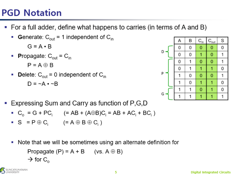
Fig.1 : PGD Notation
PGD (Propagate, Generate, Delete) notation is a method used to describe carry behavior in a full adder based only on the input bits A and B.
Generate (\(\text{G} = \text{A} \cdot \text{B}\)): The adder generates a carry regardless of the input carry, so \(\text{C}_{out}=1\). Propagate (\(\text{P} = \text{A} \oplus \text{B}\)): The input carry is propagated to the output, so \(\text{C}_{out}=\text{C}_{in}\).
Delete (\(\text{D} = \overline{A}\cdot\overline{B}\)): The carry is deleted regardless of the input carry, so \(\text{C}_{out}=0\).
Using PGD notation, the carry and sum outputs can be expressed as:
\[\text{C}_{out}=\text{G}+\text{P} \cdot \text{C}_{in}\] \[\text{S}=\text{P} \oplus \text{C}_{in}\]This notation simplifies carry analysis and is widely used in high-speed adder designs such as carry-lookahead and parallel-prefix adders.
Look Ahaed Adder
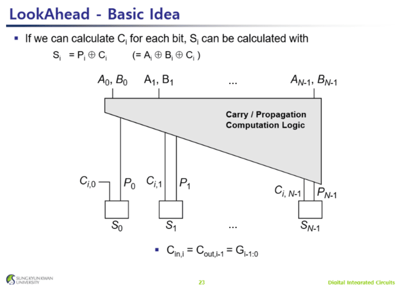
Fig.2 : Look Ahaed Adder
The basic idea of carry lookahead logic. Instead of waiting for the carry signal to ripple through each bit one by one, the circuit computes all carry signals \(\text{C}_{i}\) in parallel using the propagate (P) and generate (G) signals. Once the carry for each bit is available, the sum can be calculated as
\(\text{S}_{i} = \text{P}_{i} \oplus \text{C}_{i} = \text{A}_{i}\oplus \text{B}_{i} \oplus\text{C}_{i}\).
The carry/propagation computation block receives all input bits (\(\text{A}_{i}, \text{B}_{i}\)) and quickly determines the carry for every stage. This parallel carry computation significantly reduces delay compared to a ripple-carry adder, making carry lookahead adders much faster for large bit-width additions.
Black Cell, Gray Cell and Buffer
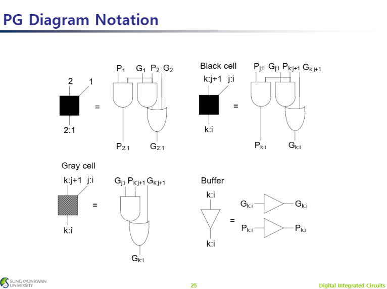
Fig.3 : Black cell, Gray cell and Buffer
There are fundamental building blocks used in parallel-prefix adders, such as the Kogge–Stone adder. These cells combine propagate (P) and generate (G) signals to efficiently compute carry information across multiple bit positions.
Black Cell: Combines two PG pairs and produces both a new propagate and a new generate signal:
\[\text{P}_{k:i} = \text{P}_{j:i} \cdot \text{P}_{k:j+1}\] \[\text{G}_{k:i}=\text{G}_{k:j+1}+\text{P}_{k:j+1} \cdot \text{G}_{j:i}\]Since it outputs both P and G, it is used in intermediate stages of the prefix network.
Gray Cell: Computes only the generate signal:
\[\text{G}_{k:i} = \text{G}_{k:j+1} + \text{P}_{k:j+1} \cdot \text{G}_{j:i}\]Because only the carry information is needed at the final stage, the propagate output is omitted, reducing hardware complexity.
Buffer: Simply forwards the existing P and G signals without modification. It is used to balance timing and maintain a regular network structure.
By repeatedly combining PG signals with black and gray cells, a parallel-prefix adder can calculate carries for all bits in parallel, achieving much lower delay than a ripple-carry adder.
Sklansky Adder
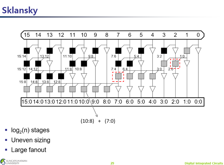
Fig.4 : Sklansky Adder
The structure of a 16-bit Sklansky parallel-prefix adder is as the above image, which is designed to compute carry signals with low logic depth. The network combines propagate (P) and generate (G) signals through a hierarchy of black and gray cells to determine carries for all bit positions.
A key advantage of the Sklansky adder is that it requires only \(\log_2(n)\) stages, allowing carry signals to be generated much faster than in a ripple-carry adder. At each stage, larger groups of bits are combined, such as (10:8) and (7:0), to form wider carry prefixes.
However, the Sklansky structure has some drawbacks. The distribution of logic is uneven, meaning that some nodes drive significantly more outputs than others. This results in large fanout, especially near the most significant bits, which can increase delay and power consumption in practical implementations. Despite this limitation, the Sklansky adder remains attractive because of its small logic depth and relatively low hardware complexity.
2. Basic Cell Design for Carry Lookahead Adder
Setup Cell
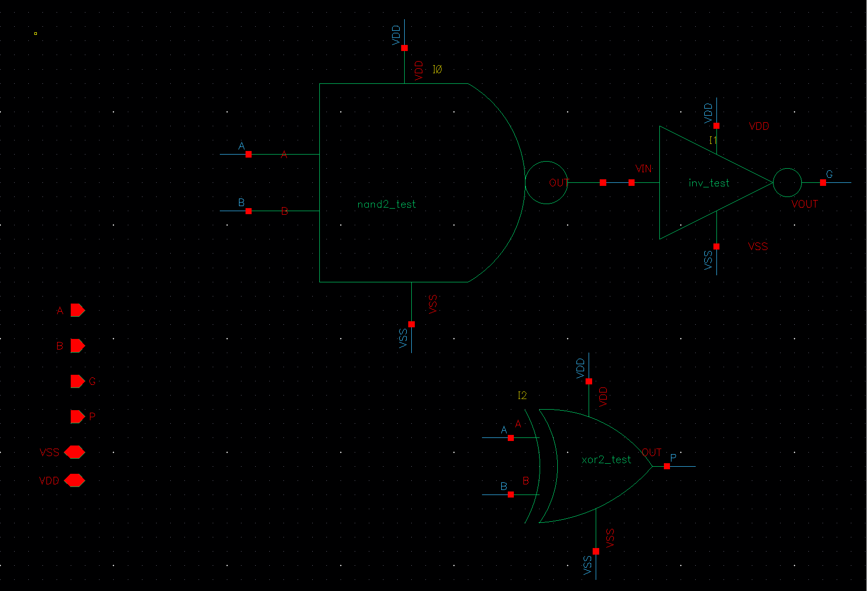
Fig.5 : Setup Cell
Carry Cell
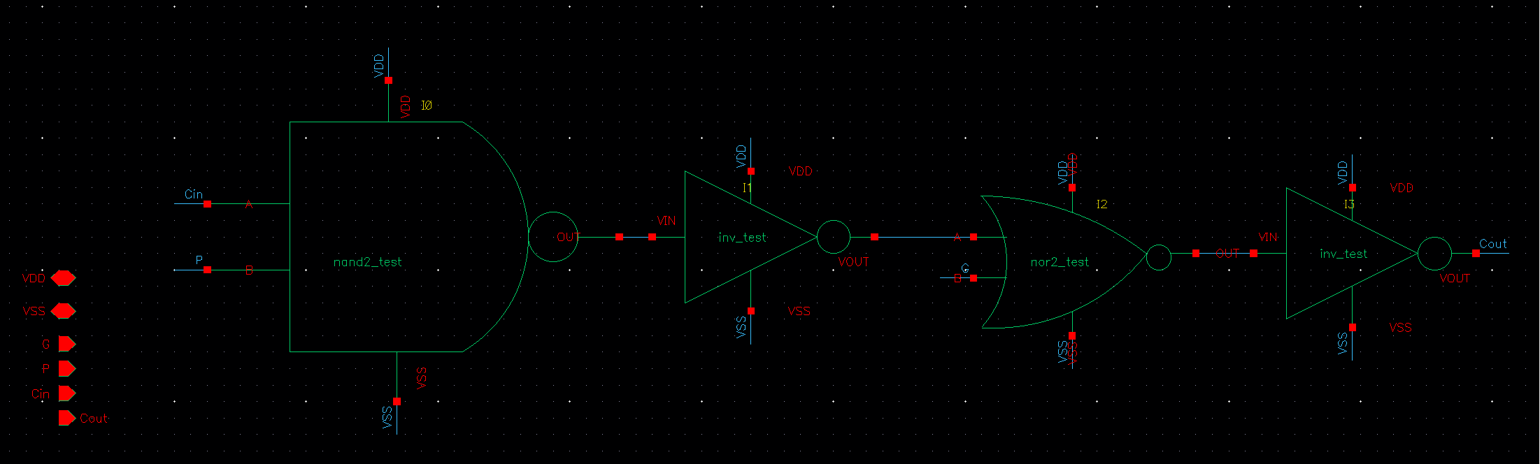
Fig.6 : Carry Cell
Sum Cell
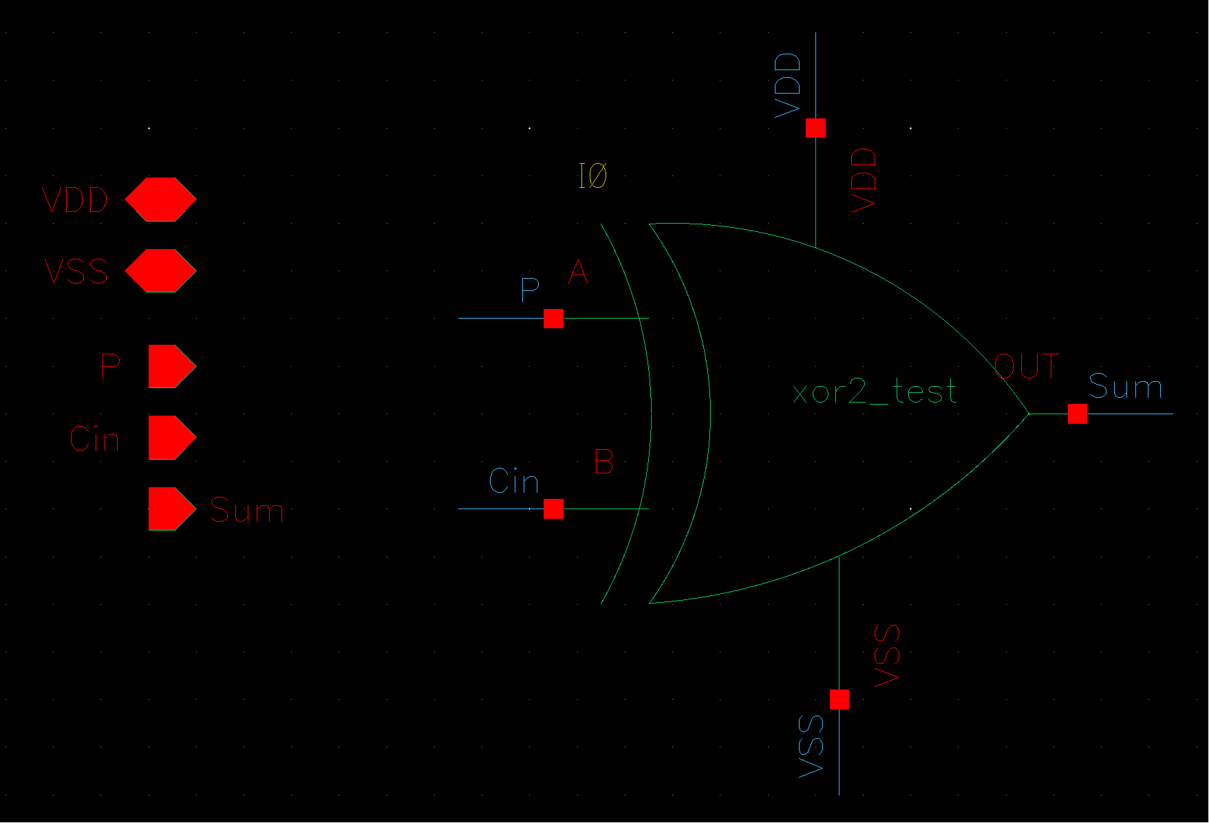
Fig.7 : Sum Cell
Black Cell
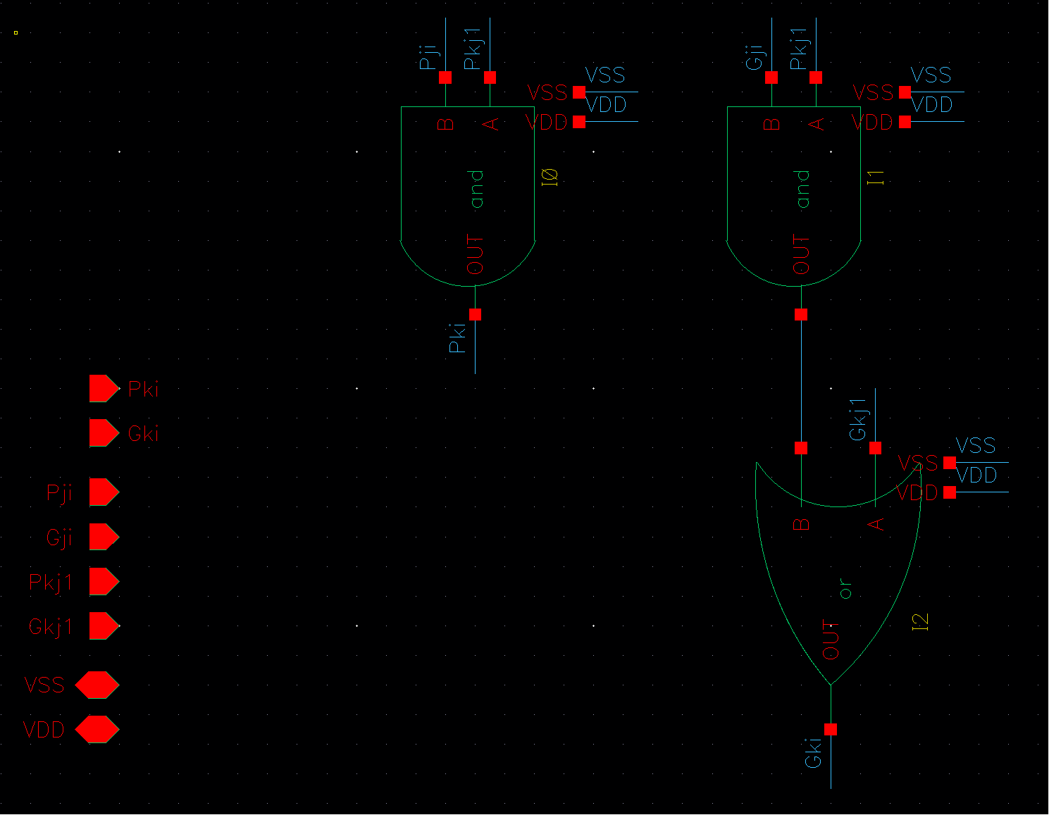
Fig.8 : Black Cell
Gray Cell
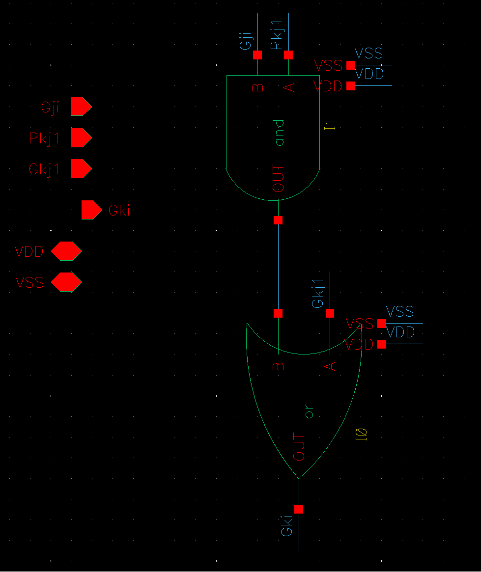
Fig.9 : Gray Cell
3. 16bit Carry Lookahead Adder Design
Sklansky Adder
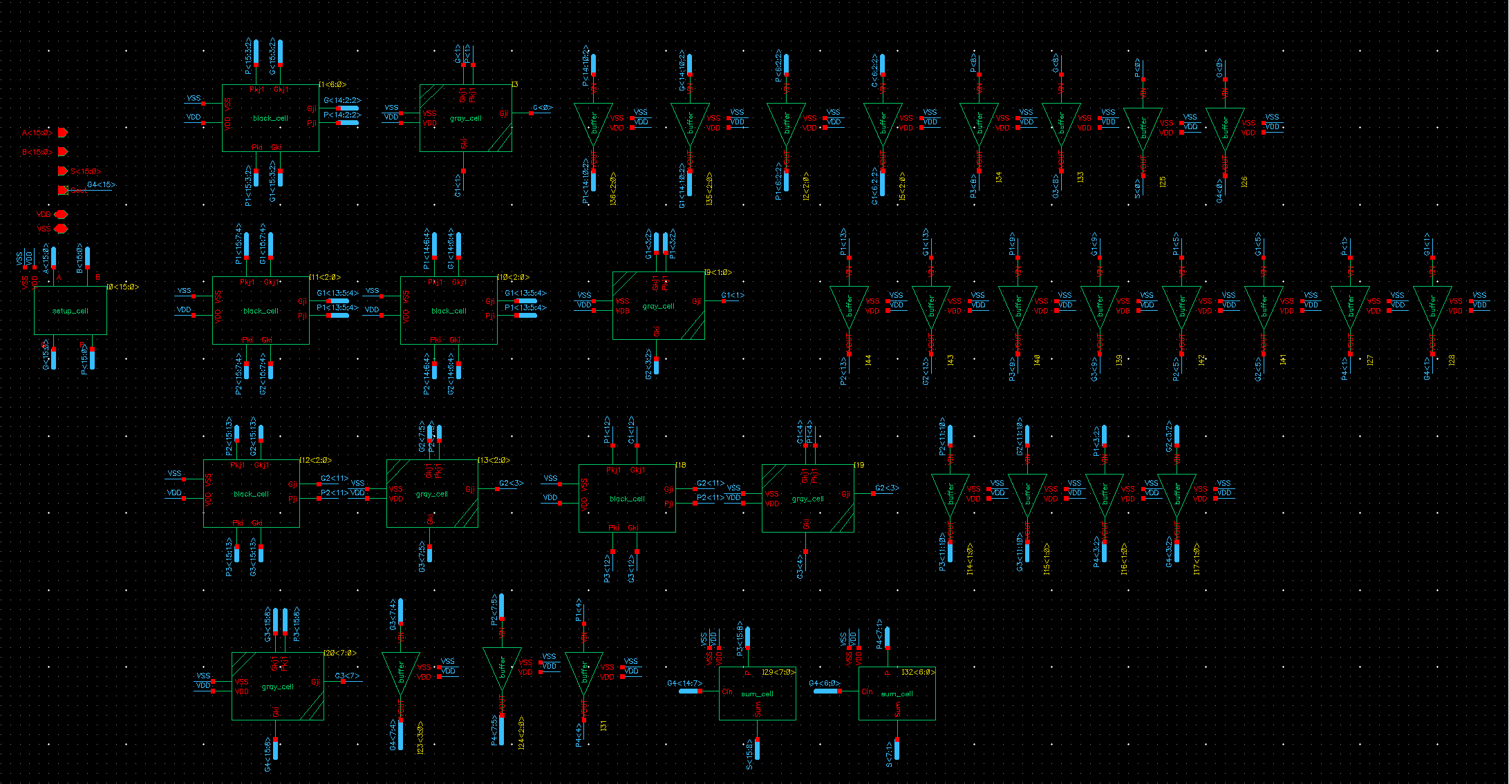
Fig.10 : Sklansky Adder
Sklansky Adder with Flip Flops
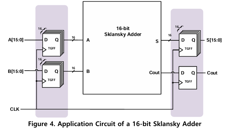
Fig.11 : Sklansky Adder with Flip Flops
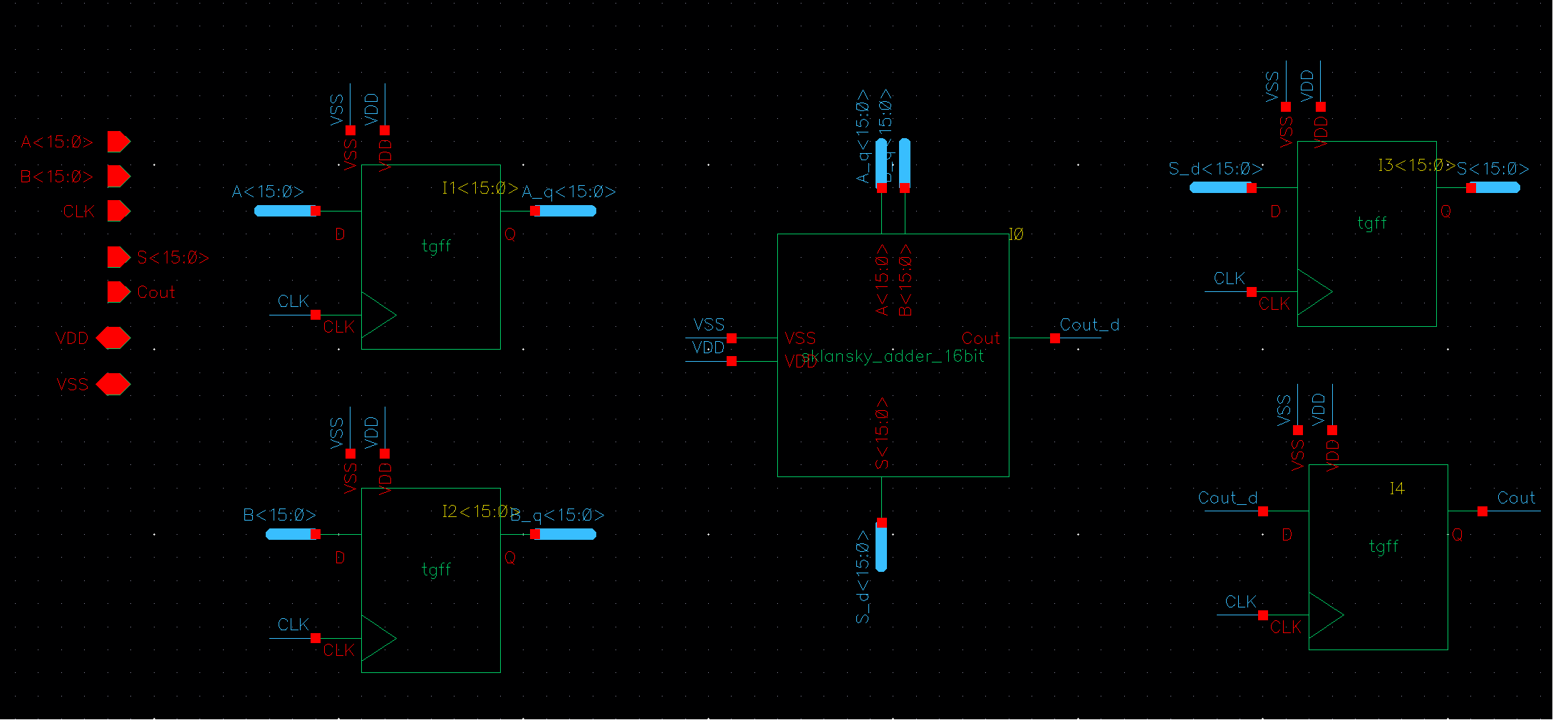
Fig.12 : Sklansky Adder with Flip Flops Design
This figure shows the application circuit used to verify the 16-bit Sklansky adder. To accurately evaluate the adder under realistic operating conditions, flip-flops (FFs) were placed at both the input and output sides of the adder.
The input flip-flops register the 16-bit operands A[15:0] and B[15:0] on the rising edge of the clock and provide stable inputs to the Sklansky adder. The adder then performs the addition and generates the sum S[15:0] and carry-out (Cout). The output flip-flops capture these results at the next clock edge, enabling synchronous operation and accurate timing measurements.
By surrounding the combinational adder with input and output registers, the circuit can be simulated and analyzed as a pipelined system, allowing the propagation delay and overall performance of the 16-bit Sklansky adder to be verified more reliably.
Functionality Verification
Case 1.
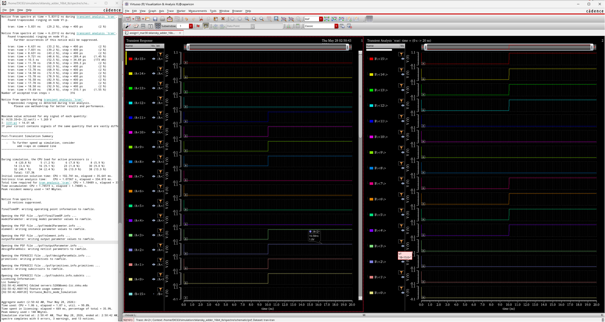
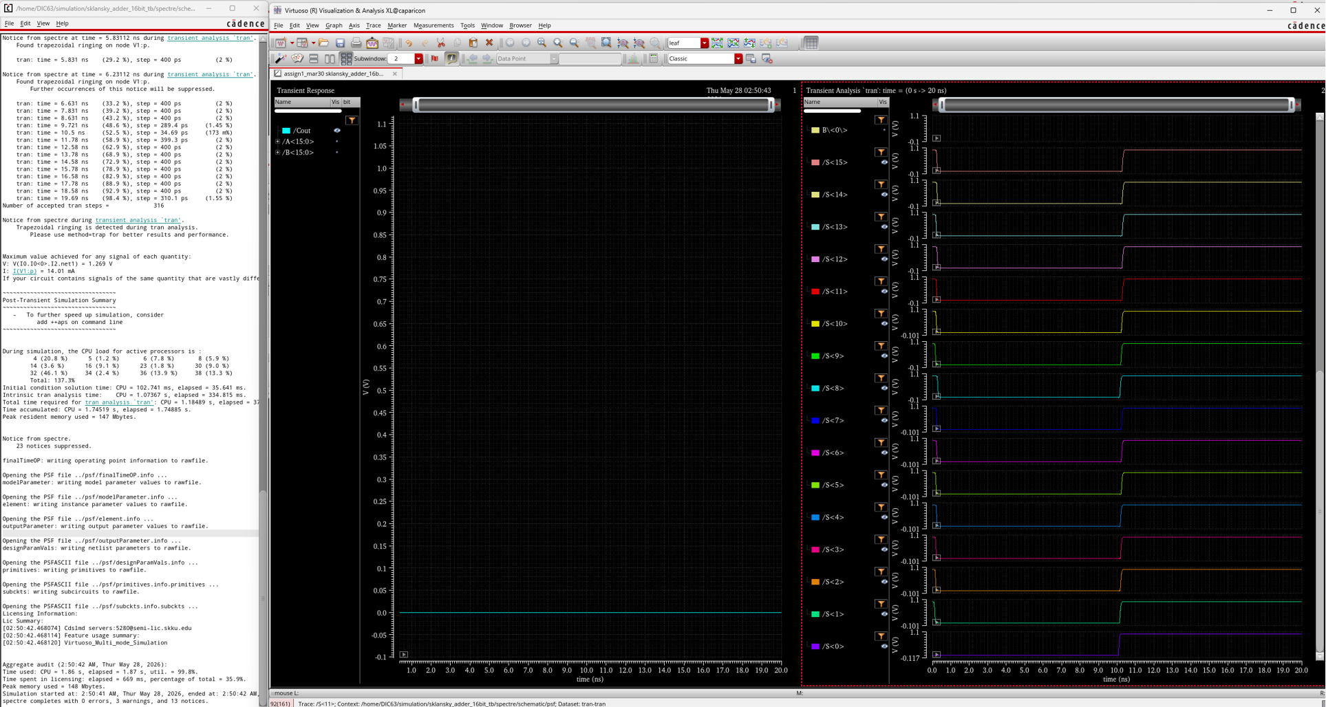
Fig. 13-14 : Case 1
A=0000_0000_0000_0000 → 0000_1111_0000_1111
B=0000_0000_0000_0000 → 1111_0000_1111_0000
S=0000_0000_0000_0000 → 1111_1111_1111_1111
Cout = 0
Case 2.
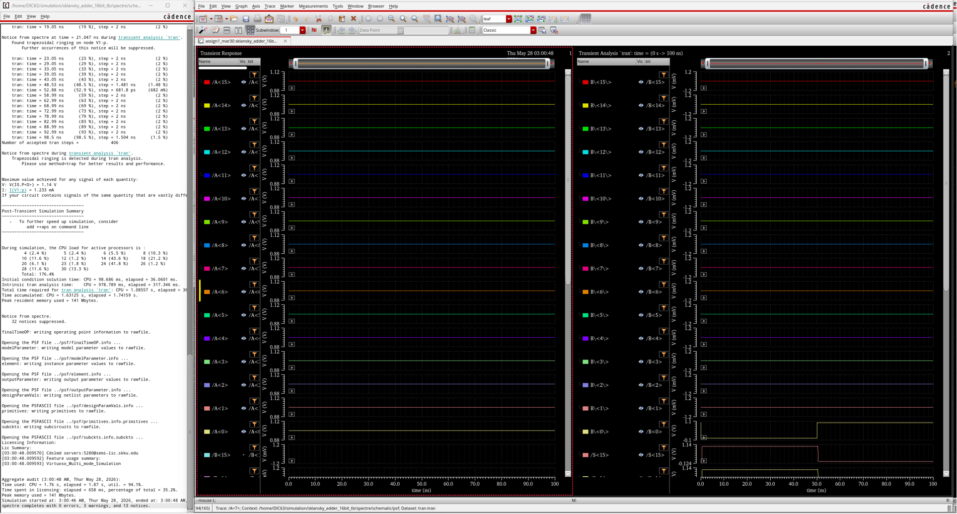
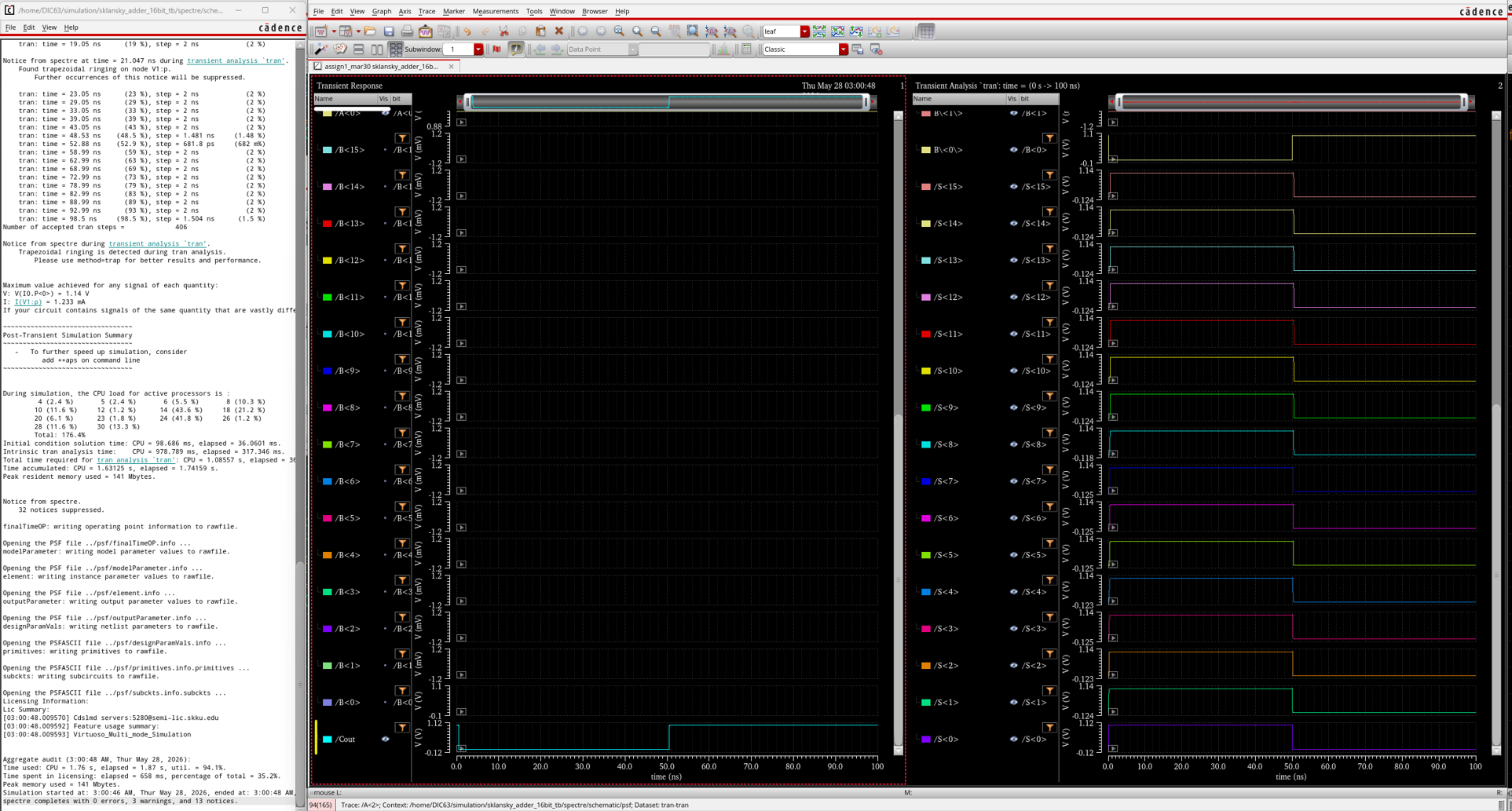
Fig. 15-16 : Case 2
A=1111_1111_1111_1111
B=0000_0000_0000_0000 → 0000_0000_0000_0001
S=1111_1111_1111_1111 → 0000_0000_0000_0000
Cout = 0 → 1
Case 3.
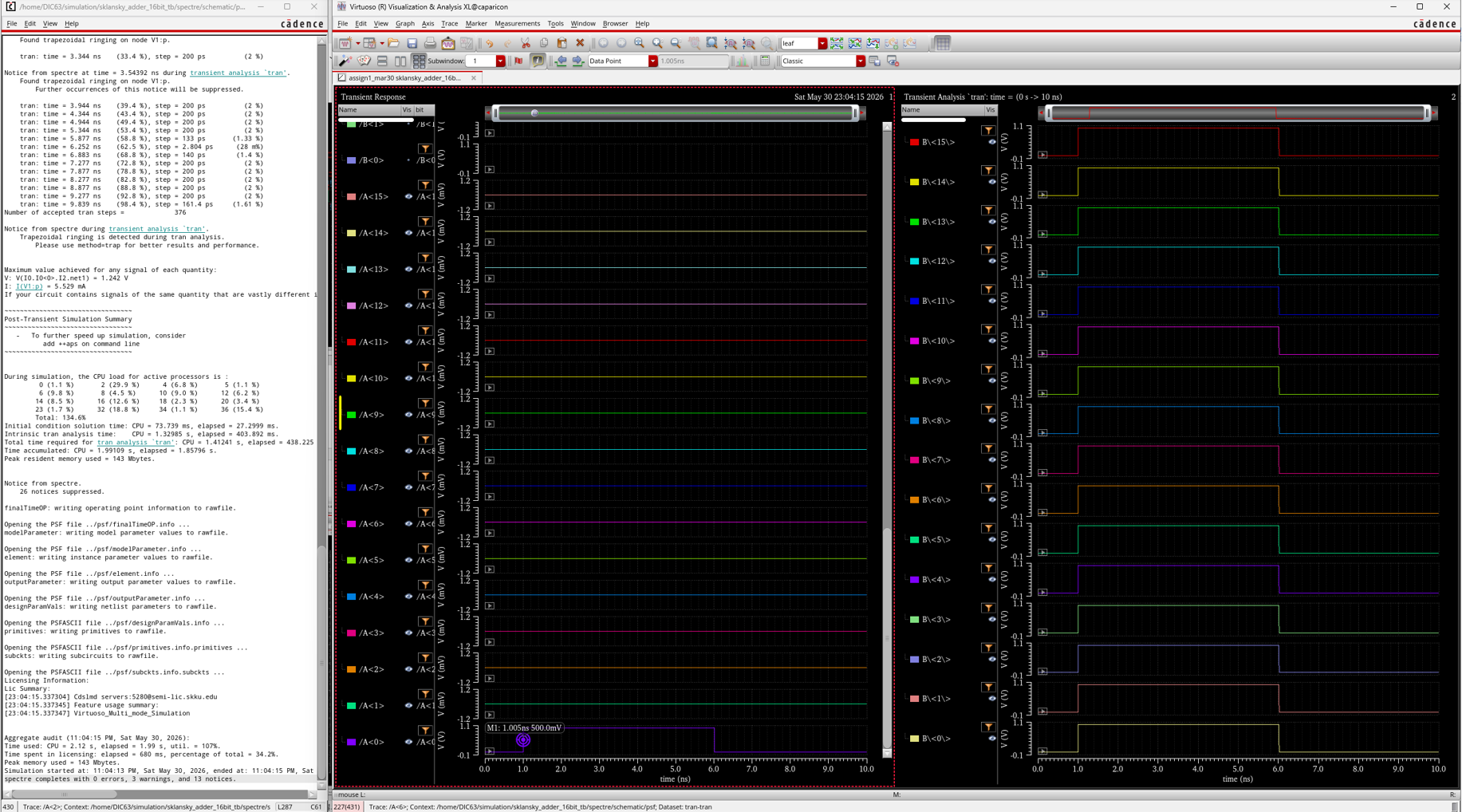
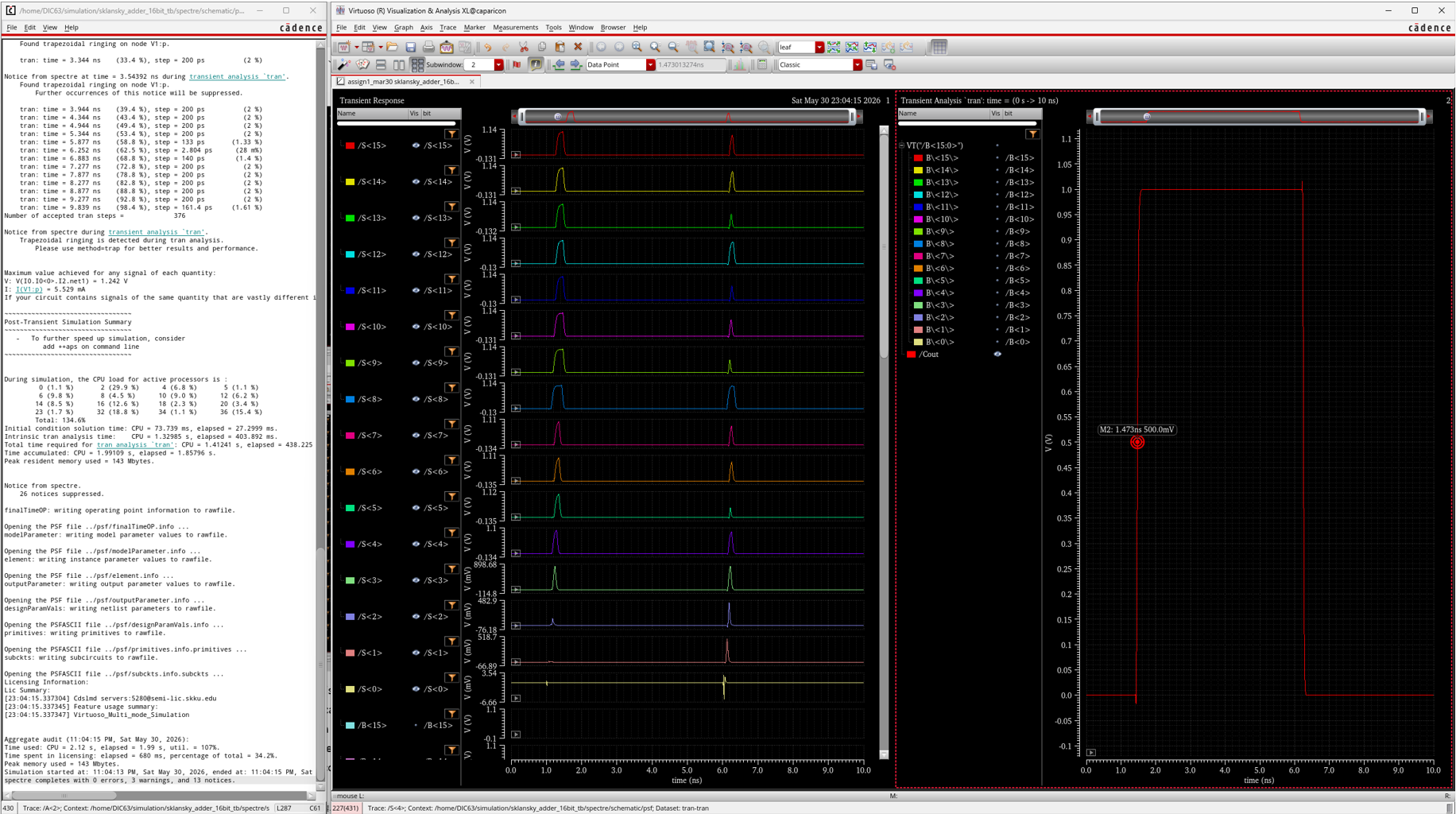
Fig. 17-18 : Case 3
A = 0000 0000 0000 0000 → 0000 0000 0000 0001
B = 0000 0000 0000 0000 → 1111 1111 1111 1111
S = 0000 0000 0000 0000 → 0000 0000 0000 0000
Cout = 0 → 1
Although the final sum output is zero, temporary glitches were observed on the sum bits during the input transition. This occurs because the propagate signals reach the sum XOR gates earlier than the carry signals generated through the prefix tree. As a result, the sum output temporarily changes before the correct carry arrives, and then settles to the correct final value. Therefore, these glitches are caused by unequal path delays in the combinational Sklansky adder and do not indicate a functional error.
This case occurs the worst case delay since it is a pattern such that a carry is generated at the least significant bit and propagated through all higher bits to the final carry-out. In this case, bit 0 generates a carry, while bits 1 through 15 are in the propagate condition. Therefore, the carry must travel through the longest prefix path of the 16-bit Sklansky adder, producing the worst-case delay at Cout.
\[\text{T}_{delay, Cout} = 1.473ns – 1.005ns = 0.468ns\]4. Layout Design of Basic cells
Setup Cell
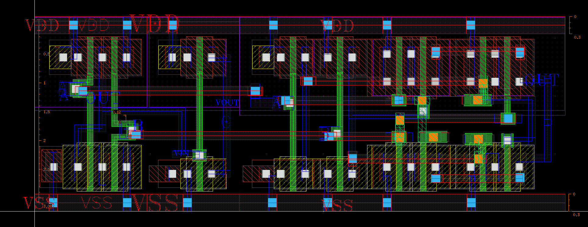
Fig.19 : Setup Cell
Carry Cell
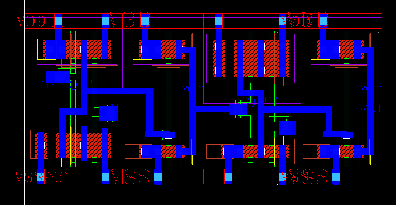
Fig.20 : Carry Cell
Sum Cell
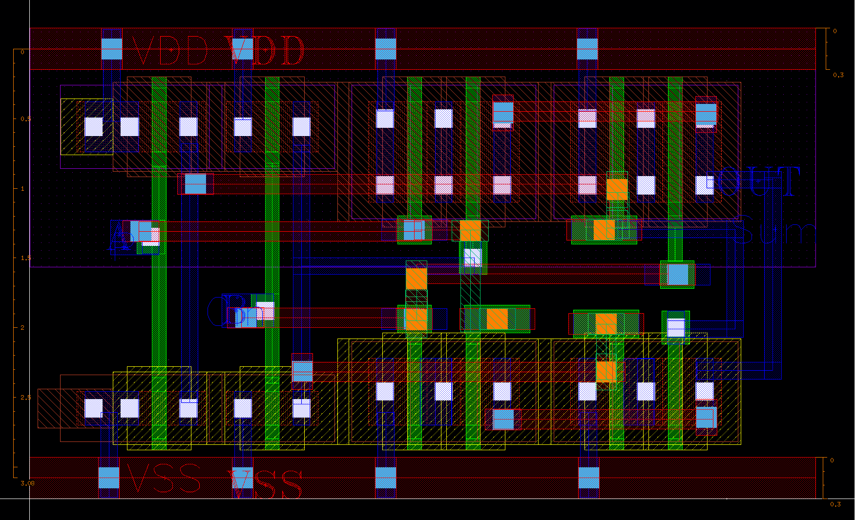
Fig.21 : Sum Cell
Black Cell
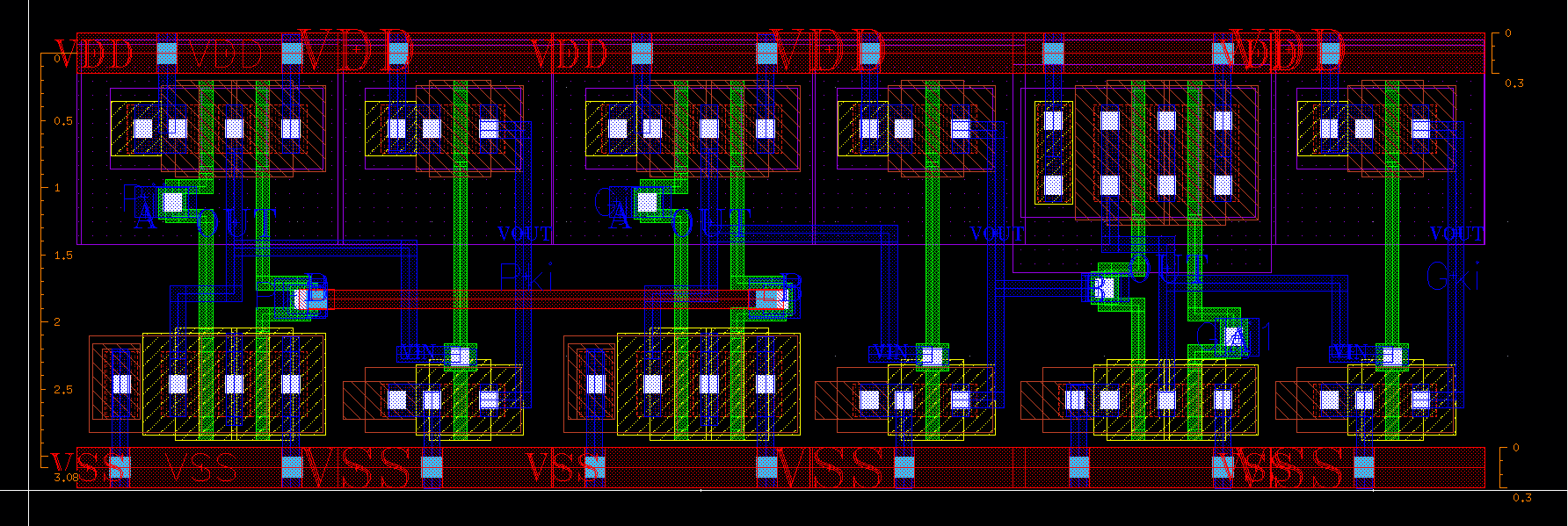
Fig.22 : Black Cell
Gray Cell
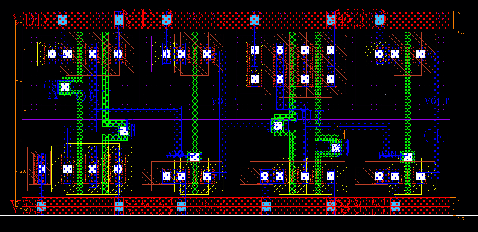
Fig.23 : Gray Cell
TGFF
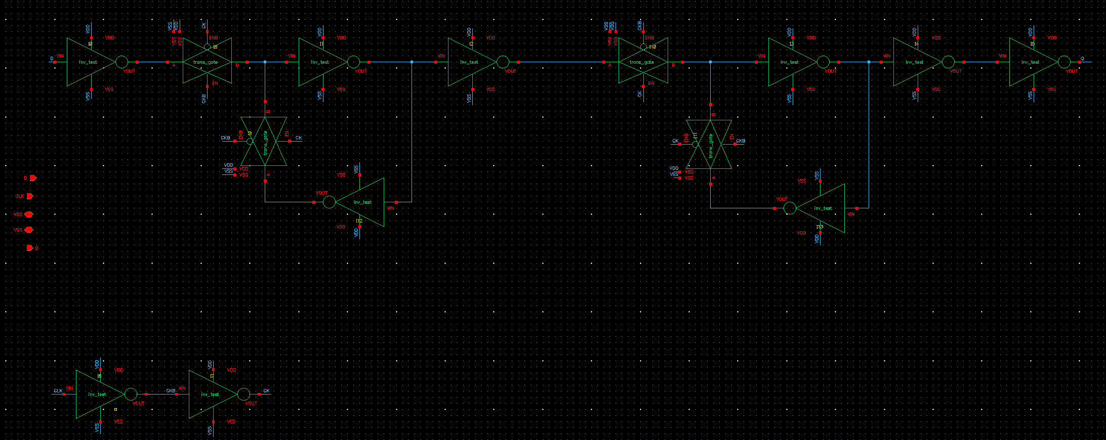
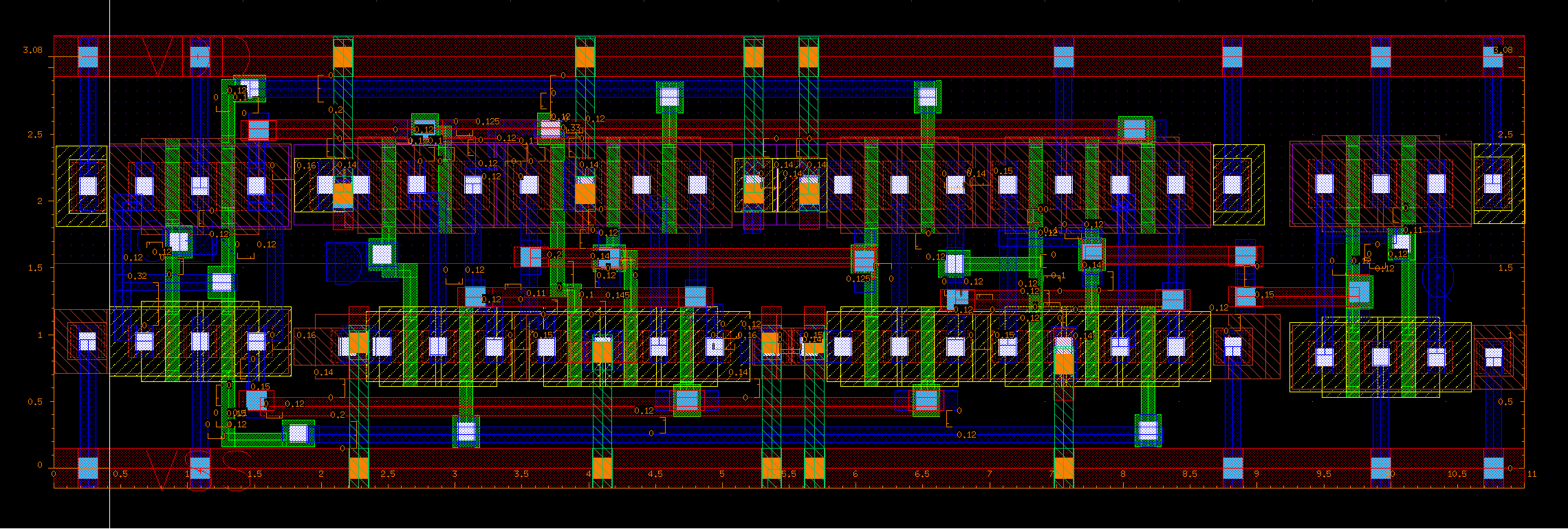
Fig.24-25 : TGFF Schematic and Layout
5. Layout Design of 16bit sklansky adder
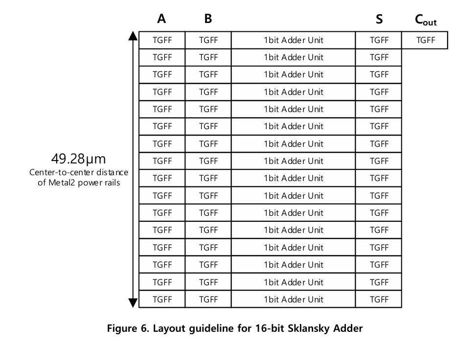
Fig.26 : Floorplan
This figure illustrates the floorplan of the 16-bit Sklansky adder, where 16 one-bit adder units are arranged vertically between input and output TGFFs to achieve a regular layout structure while satisfying the 49.28 μm center-to-center spacing requirement of the Metal2 power rails.
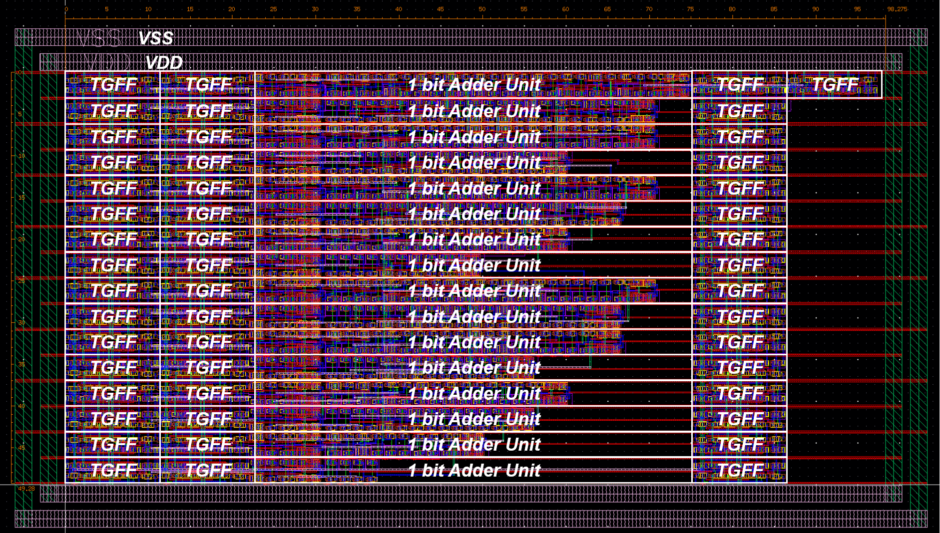
Fig.27 : Final Layout
This figure shows the final layout implementation of the 16-bit Sklansky adder in Cadence Virtuoso, where the TGFFs are placed on both sides of the adder core and the routing is completed while maintaining the required power rail structure and layout constraints.